Download

1 / 67
670 likes | 824 Vues
Lecture 6: Capital Budgeting Part 1. C. L. Mattoli. This week. In the book, chapter 8. Intro. In the beginning of the course, we looked at the 3 main decisions that financial managers of a company need to make: capital structure, capital budgeting, and WC management.

E N D
Lecture 6: Capital Budgeting Part 1 C. L. Mattoli
This week • In the book, chapter 8.
Intro • In the beginning of the course, we looked at the 3 main decisions that financial managers of a company need to make: capital structure, capital budgeting, and WC management. • Capital budgeting or allocation is, probably, the most important of the 3 since it will determine the very character of the business. • Also, since the capital budgeting decisions are basically what the business invests its money in, we also call it the investment decision of the firm.
Intro • There will be many potential investment opportunities facing the firm. • The firm will need to replace old equipment and it might decide to purchase new equipment for a new business or to enter a new market. • These decisions are not only important, to begin with, but they cover a long future time horizon and they are not easy to reverse.
Decision under Constraint • The investment decision must be made subject to a number of constraints. • One is, obviously, that the firm will have limited funds to invest. • There will be no information about market value of the project. • More important, though, is that the goal of management is to maximize owner’s value in the business. • Of course, even that goal must be carried out under the other constraints of the real world.
Value • We have learned that the proper way to value things is using DFCF methods. • In the present context, then, we should value potential projects for the firm by discounting the expected cash flows of the project. • Projects will also have initial investment, startup costs. • Thus, our method of valuing a project will be to value it on DFCF, then, compare that value to how much it will cost to start the project.
Value • This is the essence of the Net present value (NPV) method of valuing business projects. • The NPV of a project is the difference between the DFCF value and the initial investment outlay (IO) , i.e.,
Whole worth more than parts • The idea behind business investment is that the whole is worth more than the parts. • A business buys a machine, adds labor and materials, and produces a final product for sale at a price above the price of inputs. • As a more common, simple example, consider buying an old house and renovating it. • You pay $100,000 for the house. You get estimates of $20,000 from the plumber, $10,000 from the electrician, $30,000 for plaster and paint.
Whole worth more than parts • Assume that you also have estimates from real estate agents that the house, if perfect, would sell for $200,000. • Then, adding your costs (assuming the time involved for the project is short and you can neglect time value), your estimated cost is $160,000 versus potential sale of $200,000. • Thus, you have combined input of materials and labor to produce extra value of $40,000 ($200,000 – $160,000).
Business investment value • As we said, previously, business investment is similar to the above example: the output is worth more than the input. • However, in the case of a business investment, there is a longer time frame for the project. • Thus, we expect multiple future cash flows, and we must account for the time value of cash flows. • Also, those future cash flows are just estimates.
Business investment value • Moreover, they are more complicated cash flows, involving estimates of future costs of inputs, like labor and materials, as well as estimated sales prices and volumes, in future years. • The original investment outlay will involve purchase of PP&E as well as estimates of other startup requirements of WC. • The final ingredient is a proper choice of the RRR that will give investors enough of a return.
A first example • Assume Craig wants to add dress making to his businesses. • He buys a sewing machine for $1,000, and he assumes that it will last for 5 years. • Craig estimates his inflows (dress sales) and outflows (costs) over the five years. • At the end of the 5 year project, Craig believes that he can resell the used sewing machine for $100 as scrap (or as a used sewing machine).
The cash flows • Assuming that the proper RRR for Craig is 15%, then, we have the situation displayed in the table, below.
The outcome • In the above table, we assume that the RRR for Craig’s businesses is 15%. • As you can see from the table, the DFCF value of the net inflows is $1,055. • Thus, the NPV = $1,055 - $1,000 = $55, which means that the project is estimated to add $55 in value to Craig’s business above his RRR over the period. • Alternatively, if NPV had turned out to be a negative value, it would subtract from the net worth of the business.
The NPV Decision Rule • From the above example and discussion, we can come up with a decision rule for using NPV. • Assume that the firm is in business and they already have a RRR demanded by their investors. • Indeed, given our discussion in Mod 4 (Securities valuation), shareholders will determine the value of the company’s stock based on DFCF valuation, using an appropriate RRR.
The NPV Decision Rule • Then, a project with a positive NPV will add value above the DFCF value of the firm, before taking on the project. • So, positive NPV projects should be accepted. • Alternatively, a negative NPV project will subtract value from the firm.
The NPV Decision Rule • Thus, negative NPV projects should be rejected. • A zero NPV project will leave the value of the firm unchanged, so it will neither add or detract from the value of the firm. • Thus, we would be neutral to taking on the project.
NPV & Risk • An implicit assumption in the NPV methodology, as we have described it, here, is that the risk of a project must be the same as the average risk of the firm. • We have chosen an “appropriate” discount rate to use in NPV that, as said earlier, is somehow connected to the rate at which investors discount the company’s CF’s to value its shares. • We have also learned, in the preceding module, that, in the marketplace for returns, there is a risk component to rates of return, in the market.
NPV & Risk • It follows that the risk that investors perceive in the firm has somehow been incorporated into their determination of the proper RRR for the firm. • As a result, when we use the RRR that is determined by those factors to calculate NPV of a project, the project must have the same risk as the general risk of the firm, or it will demand a different RRR.
NPV & Risk • That can be a pretty stringent requirement, if you consider the scope of projects and the scope of some firms. • For example, a new product would be a riskier than average venture. • On the other hand, a company that has a division that makes military tanks and another that makes chopsticks. • In such a company, the average risk will be different from the risks of each of its divisions.
NPV & Risk • Indeed, the NPV method must be revised to include different RRR’s for risks that are greater or less than average. • That kind of patch can be achieved by a number of formal and semi-formal means. • We leave further discussion of this to later.
A note on spreadsheet functions • It is nice to have a bunch of built-in functions in excel and other spreadsheet programs, but you should be on your guard. • In some cases, like for variance, which we shall cover later, there are several functions, and you should use the help function to find the one with the definition that you really want.
A note on spreadsheet functions • In the case of NPV, the NPV function, in excel, for example, is not the same as our definition. The excel function is actually just PV of multiple cash flows. • Thus, if you use a spreadsheet and you need to calculate NPV, you can use the NPV function, but you will have to additionally subtract out the initial investment outlay. Then, you will get the actual correct NPV, according to the true definition.
Payback Period: a non-DFCF rule • There are a number of other decision rules for investment. • The first one that we cover is the payback period, which does not account for time value. • Payback period is a natural concept that is examined in many different investment contexts. • In investment, we pay out money to buy an investment: our initial investment outlay.
Payback Period: a non-DFCF rule • The payback period for an investment is the amount of time, into the future, at which we, basically, break even, not accounting for time value, on our initial outlay. • Thus, to find the payback period, we subtract each years cash flow from the initial investment until it is completely recovered.
Payback Period: a non-DFCF rule • In practice, the investment will probably not be recovered in an integral number of years, but, instead, there will be a leftover amount in one year, which will be paid off in a fraction of a year. • For example, a payback period might be in 3 years, 4 months = 3 1/3 years. • In the next slide, we show the payback period calculation for our earlier project.
Payback Period Example • The payback period is over 3 years but under 4. It is 100/300 = 1/3 year over 3 years. 100/300 = 1/3
Payback Example • In the example, we subtract year after year of cash inflows from the original outflow. • It takes 3 years of $300 of inflows to cover $900 of the initial $1,000 outflow. • Then, there is only $100 left, and that is less than year 4’s cash flow. • So, we take the leftover $100 and divide it by year 4’s cash flow to find out what portion of a year it takes to cover the leftover. • Thus, our payback period is 3 1/3 years.
Payback Decision Rule • As the payback period (PBP) analysis is not formal, to begin with, being a non-DFCF tool, the decision rule is not a hard and fast rule. • Companies simply choose a rather arbitrary number of years, usually just a few, as an acceptable PBP. • The rule is, then, accept projects that have PBP’s equal to or less than the stated PBP of the company, and reject those that take more than the standard to pay back.
Pros & Cons of Payback • PBP neglects time value and makes an arbitrary cutoff hurdle rate for projects. • If there is only one hurdle rate for PBP, then, the riskiness of projects is also ignored. • One of the most salient faults of PBP is that it completely disregards any cash flows that come after break-even, i.e., (forgetting about time value) profits.
Pros & Cons of Payback • In that regard, it really neglects any more than just recovering your initial investment, which misses the very spirit of investment: to make a decent return on investment. • Many established and proper companies do use PBP, either as a supplemental number for decisions or for small projects. • The latter case is due to the costs of coming up with detailed estimates on which to bases more formal analyses, like NPV.
Pros & Cons of Payback • Having a short PBP, like 2 years, will bias acceptance to projects that pay themselves off, fast, and free up cash. • It should also tend to limit losses. • In the end, just as in any method of analyzing the future, we have to use estimates that might be so wrong, and that will be especially true as the years into the future increase. The PBP has a natural bias to the early years.
Average Accounting Return • Another non-DFCF method is called the average accounting return (AAR) of a project or the accounting rate of return (ARR). • There are a number of different definitions of AAR, but they all have the general form: [average accounting profits from investment]/[average accounting value of investment]. • In this course, we shall use the specific definition: average net income/average book value.
ARR Example • Consider renting space for a dress shop. • Assume that renovation an fittings cost $100,000. • The building owner will only give you a 5 year lease, so the store will close at that time. • Assume that the initial investment is depreciated over the 5 years, straight-line.
ARR Example • Then, the average investment will be [$100,000 (IIO) + $0 (terminal BV)]/2 = $50,000. • The estimated net incomes for the 5 years are $50,000, $75,000, $25,000, $0, and – $10,000. • Then, the average profit is [$50K + $75K + $25K + $0 – $10K]/5 = $28,000. • Thus AAR = $28,000/$50,000 = 56%
ARR Decision Rule • Just like the PBP, the ARR method is a rule of thumb (a heuristic, in the newer language of behavioral finance). • The choice of a hurdle rate is somewhat arbitrary. • Given a specified hurdle rate for ARR, then, accept projects that make the hurdle, and reject projects that do not make the hurdle (or target) rate or benchmark.
ARR Expose • ARR uses accounting numbers so it will not give a representation of return that has meaning in the economic sense. • The numbers used in ARR do not account for time value, so they mix numbers from different times. • The numbers, moreover, are not even cash flows: they are profits. • Like PBP, a benchmark rate is arbitrary, although we could compute the ARR for the firm as a whole and use that. • Advantage: easy to compute wil readily-available accounting numbers.
Internal Rate of Return • A second DFCF method that we shall examine is internal rate of return (IRR). • We already encountered the concept of IRR when we looked at bonds: the IRR solves the coupon bond equation for YTM. • The IRR method is also related to NPV. • With NPV we begin with a given value for RRR, and we compare the DFCF from the investment with the price, IIO, that we pay for the investment.
Internal Rate of Return • On the other hand, IRR finds the RRR that makes DFCF exactly equal to IIO. • In other words, IRR is the rate of return that equates the present value of the project’s cash flows to the initial outlay of the project. • Thus, we can write the equation form of IRR as: • Then, the requiredrate of return that makes NPV=0 is the IRR.
Finding IRR • As noted in our discussion of finding YTM, IRR can not, usually, be found, directly, but must be found either with a financial function on calculator or spreadsheet or by trial and error. • In our earlier example calculation of NPV, we used RRR = 15%, and we found that NPV was positive. • That means, if we were setting out to find IRR by trail and error, we know that the value is greater than 15% because that value of RRR made the sum of DFCF larger than the IO. • We used the IRR function in excel to find the IRR for our dress-making project and found IRR = 17.23%.
RRR vs. NPV • In the chart below we show RRR vs. NPV for our project, known as an NPV profile
Finding IRR using excel • As mentioned earlier, be careful when using spreadsheet functions to understand what they are and how to use them to get the answers that you need. • The excel function is of the form IRR(values, guess), e.g., IRR(E16:J16,0.1) • At least one of the values must be negative and one positive. • The guess is any number: it just needs an RRR to start the trial and error.
IRR Decision Rules • Since IRR is the return that makes NPV=0, we can translate the decision rules for NPV into IRR. • Thus, if IRR is greater than the hurdle RRR, accept the project. • If it is less, reject. • If IRR = the hurdle rate, the position is neutral. • This is displayed graphically, in the chart in the slide, above.
More detailed information • The general rules for using IRR were given in the preceding slide, but we must embellish them. • First, the project must be an independent project, not dependent on anything else. • If CF’s are negative in more than the initial year, the IRR problem has multiple solutions, not just one, which makes a decision difficult.
More detailed information • Even the evenness of CF’s can affect the usefulness of IRR, for example, if CF’s are weighted in the early versus the later years. • A general disadvantage of IRR over NPV is that when a multi-year project has a certain IRR, the implicit assumption in PV DFCF is that intermediate year CF’s must be reinvested at the IRR rate.
More detailed information • NPV assumes that intermediate CF’s are reinvested at the RRR, which, since the RRR is the return that is being achieved by projects of the firm, in general, there should be reinvestment opportunities, in the future, at that general rate. • However, for IRR, if the IRR is substantially above the RRR, it is not reasonable to assume that we can reinvest at that high rate through other future projects.
Mutually Exclusive Projects • Projects can be mutually exclusive (ME). • That means choosing one but not both (or all). • For example, you want to buy a new computer for your business. You evaluate the CF’s of using IBM, HP, or Lenovo. • In the end, you need only one computer system, so, choosing one eliminates the others.
Mutually Exclusive Projects • Often, the ME nature of projects is subtle, and a problem might not tell you that the projects are ME ... Figuring that out will be part of the problem. • If projects are not ME, they are independent. • Once that you figure out that a set of projects is ME, then, the decision will be to choose the one that has the highest NPV or IRR or whatever your criterion is.
ME example • CF’s for two projects, B & C, are shown, below. • The NPV of B is $147 and C is $106, using a 10% RRR. • IRR’s for the projects are 17.01% for B and 13.06% for C.