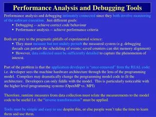
Download
1 / 94
940 likes | 963 Vues
This presentation discusses the concepts, definitions, and tools used for conducting performance analysis in the field of computer science. It covers topics such as instrumentation, monitoring, and analysis, as well as specific tools like PAPI, ompP, and IPM. The goal is to improve the performance of computer systems and solve problems faster and more efficiently.

E N D
Performance Analysis ToolsCS267, March 30, 2010 Karl Fuerlinger fuerling@eecs.berkeley.edu With slides from David Skinner, Sameer Shende, Shirley Moore, Bernd Mohr, Felix Wolf, Hans Christian Hoppe and others.
Outline • Motivation • Concepts and definitions • Instrumentation, monitoring, analysis • Some tools and their functionality • PAPI – access to hardware performance counters • ompP – profiling OpenMP code • IPM – monitoring message passing applications • (Backup Slides) • Vampir • Kojak/Scalasca • TAU
Motivation • Performance analysis is important • For HPC: computer systems are large investments • Procurement: O($40 Mio) • Operational costs: ~$5 Mio per year • Power: 1 MWyear ~$1 Mio • Goals: • Solve larger problems (new science) • Solve problems faster (turn-around time) • Improve error bounds on solutions (confidence)
Concepts and Definitions • The typical performance optimization cycle Code Development Functionally complete and correct program Instrumentation Measure Analyze Modify / Tune Complete, cor-rect and well- performing program Usage / Production
source code instrumentation preprocessor instrumentation User-level abstractions problem domain source code instrumentation compiler instrumentation object code libraries linker OS executable instrumentation instrumentation runtime image instrumentation instrumentation VM performancedata run Instrumentation • Instrumentation := adding measurement probes to the code in order to observe its execution • Can be done on several levels and ddifferent techniques for different levels • Different overheads and levels of accuracy with each technique • No application instrumentation needed: run in a simulator. E.g., Valgrind, SIMICS, etc. but simulation speed is an issue
Instrumentation – Examples (1) • Library Instrumentation: • MPI library interposition • All functions are available under two names: MPI_Xxx and PMPI_Xxx, • MPI_Xxx symbols are weak, can be over-written by interposition library • Measurement code in the interposition library measures begin, end, transmitted data, etc… and calls corresponding PMPI routine. • Not all MPI functions need to be instrumented
Pre-processor Modified (instrumented) source code Orignialsource code POMP_Parallel_fork [master]#pragma omp parallel { POMP_Parallel_begin [team] /* user code in parallel region */ POMP_Barrier_enter [team] #pragma omp barrier POMP_Barrier_exit [team] POMP_Parallel_end [team]}POMP_Parallel_join [master] Instrumentation – Examples (2) • Preprocessor Instrumentation • Example: Instrumenting OpenMP constructs with Opari • Preprocessor operation • Example: Instrumentation of a parallel region This approach is used for OpenMP instrumentation by most vendor-independent tools. Examples: TAU/Kojak/Scalasca/ompP #pragma omp parallel { /* user code in parallel region */ } Instrumentation added by Opari
Instrumentation – Examples (3) • Source code instrumentation • User-added time measurement, etc. (e.g., printf(), gettimeofday()) • Think twice before you roll your own solution, many tools expose mechanisms for source code instrumentation in addition to automatic instrumentation mechanisms Instrument program phases: • Initialization • main loop iteration 1,2,3,4,... • data post-processing • Pragma and pre-processor based #pragma pomp inst begin(foo)// application code #pragma pomp inst end(foo) • Macro / function call basedELG_USER_START("name");// application code • ELG_USER_END("name");
Instrumentation – Examples (4) • Compiler Instrumentation • Many compilers can instrument functions automatically • GNU compiler flag: -finstrument-functions • Automatically calls functions on function entry/exit that a tool can capture • Not standardized across compilers, often undocumented flags, sometimes not available at all • GNU compiler example: void __cyg_profile_func_enter(void *this, void *callsite) { /* called on function entry */ } void __cyg_profile_func_exit(void *this, void *callsite) { /* called just before returning from function */ }
Instrumentation – Examples (5) • Binary Runtime Instrumentation • Dynamic patching while the program executes • Example: Paradyn tool, Dyninst API • Base trampolines/Mini trampolines • Base trampolines handle storing current state of program so instrumentations do not affect execution • Mini trampolines are the machine-specific realizations of predicates and primitives • One base trampoline may handle many mini-trampolines, but a base trampoline is needed for every instrumentation point • Binary instrumentation is difficult • Have to deal with • Compiler optimizations • Branch delay slots • Different sizes of instructions for x86 (may increase the number of instructions that have to be relocated) • Creating and inserting mini trampolines somewhere in program (at end?) • Limited-range jumps may complicate this Figure by Skylar Byrd Rampersaud • PIN: Open Source dynamic binary instrumenter from Intel
Measurement • Profiling vs. Tracing • Profiling • Summary statistics of performance metrics • Number of times a routine was invoked • Exclusive, inclusive time • Hardware performance counters • Number of child routines invoked, etc. • Structure of invocations (call-trees/call-graphs) • Memory, message communication sizes • Tracing • When and where events took place along a global timeline • Time-stamped log of events • Message communication events (sends/receives) are tracked • Shows when and from/to where messages were sent • Large volume of performance data generated usually leads to more perturbation in the program
Measurement: Profiling • Profiling • Helps to expose performance bottlenecks and hotspots • 80/20 –rule or Pareto principle: often 80% of the execution time in 20% of your application • Optimize what matters, don’t waste time optimizing things that have negligible overall influence on performance • Implementation • Sampling: periodic OS interrupts or hardware counter traps • Build a histogram of sampled program counter (PC) values • Hotspots will show up as regions with many hits • Measurement: direct insertion of measurement code • Measure at start and end of regions of interests, compute difference
Profiling: Inclusive vs. Exclusive Time • Inclusive time for main • 100 secs • Exclusive time for main • 100-20-50-20=10 secs • Exclusive time sometimes called “self” time • Similar definitions for inclusive/exclusive time for f1() and f2() • Similar for other metrics, such as hardware performance counters, etc int main( ) { /* takes 100 secs */ f1(); /* takes 20 secs */ /* other work */ f2(); /* takes 50 secs */ f1(); /* takes 20 secs */ /* other work */ }
void master { trace(ENTER, 1); ... trace(SEND, B); send(B, tag, buf); ... trace(EXIT, 1); } 1 2 3 master worker ... event location context time 68 64 62 ... 69 ... 58 60 B B B A A A ENTER SEND ENTER EXIT EXIT RECV A 1 2 1 B 2 void worker { trace(ENTER, 2); ... recv(A, tag, buf); trace(RECV, A); ... trace(EXIT, 2); } Tracing Example: Instrumentation, Monitor, Trace Event definitions Process A: timestamp MONITOR Process B:
1 2 3 master worker ... 69 ... 60 64 68 58 62 ... A A B B B A EXIT RECV ENTER EXIT ENTER SEND 1 B 2 1 A 2 A 70 68 64 60 58 62 66 Tracing: Timeline Visualization main master worker B
Measurement: Tracing • Tracing • Recording of information about significant points (events) during program execution • entering/exiting code region (function, loop, block, …) • thread/process interactions (e.g., send/receive message) • Save information in event record • timestamp • CPU identifier, thread identifier • Event type and event-specific information • Event trace is a time-sequenced stream of event records • Can be used to reconstruct dynamic program behavior • Typically requires code instrumentation
Performance Data Analysis • Draw conclusions from measured performance data • Manual analysis • Visualization • Interactive exploration • Statistical analysis • Modeling • Automated analysis • Try to cope with huge amounts of performance by automation • Examples: Paradyn, KOJAK, Scalasca, Periscope
Trace File Visualization • Vampir: timeline view • Similar other tools: Jumpshot, Paraver 1 2 3
Trace File Visualization • Vampir/IPM: message communication statistics
3D performance data exploration • Paraprof viewer (from the TAU toolset)
Automated Performance Analysis • Reason for Automation • Size of systems: several tens of thousand of processors • LLNL Sequoia: 1.6 million cores • Trend to multi-core • Large amounts of performance data when tracing • Several gigabytes or even terabytes • Not all programmers are performance experts • Scientists want to focus on their domain • Need to keep up with new machines • Automation can solve some of these issues
Automation - Example • „Late sender“ pattern • This pattern can be detected automatically by analyzing the trace
Outline • Motivation • Concepts and definitions • Instrumentation, monitoring, analysis • Some tools and their functionality • PAPI – access to hardware performance counters • ompP – profiling OpenMP code • IPM – monitoring message passing applications • (Backup Slides) • Vampir • Kojak/Scalasca • TAU
Hardware Performance Counters • Specialized hardware registers to measure the performance of various aspects of a microprocessor • Originally used for hardware verification purposes • Can provide insight into: • Cache behavior • Branching behavior • Memory and resource contention and access patterns • Pipeline stalls • Floating point efficiency • Instructions per cycle • Counters vs. events • Usually a large number of countable events (several hundred) • On a small number of counters (4-18) • PAPI handles multiplexing if required
What is PAPI • Middleware that provides a consistent and efficient programming interface for the performance counter hardware found in most major microprocessors. • Countable events are defined in two ways: • Platform-neutral Preset Events (e.g., PAPI_TOT_INS) • Platform-dependent Native Events (e.g., L3_CACHE_MISS) • Preset Events can be derived from multiple Native Events(e.g. PAPI_L1_TCM might be the sum of L1 Data Misses and L1 Instruction Misses on a given platform) • Preset events are defined in a best-effort way • No guarantees of semantics portably • Figuring out what a counter actually counts and if it does so correctly can be hairy
PAPI Hardware Events • Preset Events • Standard set of over 100 events for application performance tuning • No standardization of the exact definitions • Mapped to either single or linear combinations of native events on each platform • Use papi_avail to see what preset events are available on a given platform • Native Events • Any event countable by the CPU • Same interface as for preset events • Use papi_native_avail utility to see all available native events • Use papi_event_chooser utility to select a compatible set of events
3rd Party and GUI Tools Low Level User API High Level User API PAPI PORTABLE LAYER PAPI HARDWARE SPECIFIC LAYER Kernel Extension Operating System Perf Counter Hardware PAPI Counter Interfaces • PAPI provides 3 interfaces to the underlying counter hardware: • A low level API manages hardware events (preset and native) in user defined groups called EventSets.Meant for experienced application programmers wanting fine-grained measurements. • A high level API provides the ability to start, stop and read the counters for a specified list of events (preset only).Meant for programmers wanting simple event measurements. • Graphical and end-user tools provide facile data collection and visualization.
PAPI High Level Calls PAPI_num_counters() get the number of hardware counters available on the system PAPI_flips (float *rtime, float *ptime, long long *flpins, float *mflips) simplified call to get Mflips/s (floating point instruction rate), real and processor time PAPI_flops (float *rtime, float *ptime, long long *flpops, float *mflops) simplified call to get Mflops/s (floating point operation rate), real and processor time PAPI_ipc (float *rtime, float *ptime, long long *ins, float *ipc) gets instructions per cycle, real and processor time PAPI_accum_counters (long long *values, int array_len) add current counts to array and reset counters PAPI_read_counters (long long *values, int array_len) copy current counts to array and reset counters PAPI_start_counters (int *events, int array_len) start counting hardware events PAPI_stop_counters (long long *values, int array_len) stop counters and return current counts
PAPI Example Low Level API Usage #include "papi.h” #define NUM_EVENTS 2 int Events[NUM_EVENTS]={PAPI_FP_OPS,PAPI_TOT_CYC}, int EventSet; long long values[NUM_EVENTS]; /* Initialize the Library */ retval = PAPI_library_init (PAPI_VER_CURRENT); /* Allocate space for the new eventset and do setup */ retval = PAPI_create_eventset (&EventSet); /* Add Flops and total cycles to the eventset */ retval = PAPI_add_events (&EventSet,Events,NUM_EVENTS); /* Start the counters */ retval = PAPI_start (EventSet); do_work(); /* What we want to monitor*/ /*Stop counters and store results in values */ retval = PAPI_stop (EventSet,values);
Using PAPI through tools • You can use PAPI directly in your application, but most people use it through tools • Tool might have a predfined set of counters or lets you select counters through a configuration file/environment variable, etc. • Tools using PAPI • TAU (UO) • PerfSuite (NCSA) • HPCToolkit (Rice) • KOJAK, Scalasca (FZ Juelich, UTK) • Open|Speedshop (SGI) • ompP (UCB) • IPM (LBNL)
LowLevelAPI HiLevelAPI PAPI Framework Layer DevelAPI DevelAPI DevelAPI PAPI Component Layer (thermal) PAPI Component Layer (CPU) PAPI Component Layer (network) Kernel Patch Kernel Patch Kernel Patch Operating System Operating System Operating System Perf Counter Hardware Perf Counter Hardware Perf Counter Hardware Component PAPI Design • Re-Implementation of PAPI w/ support for multiple monitoring domains
Outline • Motivation • Concepts and definitions • Instrumentation, monitoring, analysis • Some tools and their functionality • PAPI – access to hardware performance counters • ompP – profiling OpenMP code • IPM – monitoring message passing applications • (Backup Slides) • Vampir • Kojak/Scalasca • TAU
OpenMP Performance Analysis with ompP • ompP: Profiling tool for OpenMP • Based on source code instrumentation • Independent of the compiler and runtime used • Tested and supported: Linux, Solaris, AIX and Intel,Pathscale, PGI, IBM, gcc, SUN studio compilers • Supports HW counters through PAPI • Uses source code instrumenter Opari from the KOJAK/Scalasca toolset • Available for download (GPL): http://www.ompp-tool.com Automatic instrumentation of OpenMP constructs, manual region instrumentation Source Code Executable ompP library Settings (env. Vars) HW Counters, output format,… Execution on parallel machine Profiling Report
Master Thread Parallel Regions OpenMP • OpenMP • Threads and fork/join based programming model • Worksharing constructs • Characteristics • Directive based (compiler pragmas, comments) • Incremental parallelization approach • Well suited for loop-based parallel programming • Less well suited for irregular parallelism (but tasking included in version 3.0 of the OpenMP specification). • One of the contending programming paradigms for the “mutlicore era”
ompP’s Profiling Report • Header • Date, time, duration of the run, number of threads, used hardware counters,… • Region Overview • Number of OpenMP regions (constructs) and their source-code locations • Flat Region Profile • Inclusive times, counts, hardware counter data • Callgraph • Callgraph Profiles • With Inclusive and exclusive times • Overhead Analysis Report • Four overhead categories • Per-parallel region breakdown • Absolute times and percentages
Profiling Data • Example profiling data Profile: R00002 main.c (34-37) (default) CRITICAL TID execT execC bodyT enterT exitT PAPI_TOT_INS 0 3.00 1 1.00 2.00 0.00 1595 1 1.00 1 1.00 0.00 0.00 6347 2 2.00 1 1.00 1.00 0.00 1595 3 4.00 1 1.00 3.00 0.00 1595 SUM 10.01 4 4.00 6.00 0.00 11132 Code: #pragma omp parallel { #pragma omp critical { sleep(1.0); } } • Components: • Source code location and type of region • Timing data and execution counts, depending on the particular construct • One line per thread, last line sums over all threads • Hardware counter data (if PAPI is available and HW counters are selected) • Data is “exact” (measured, not based on sampling)
Flat Region Profile (2) • Times and counts reported by ompP for various OpenMP constructs Ends with T: time Ends with C: count Main = enter + body + barr + exit
Callgraph • Callgraph View • ‘Callgraph’ or ‘region stack’ of OpenMP constructs • Functions can be included by using Opari’s mechanism to instrument user defined regions: #pragma pomp inst begin(…), #pragma pomp inst end(…) • Callgraph profile • Similar to flat profile, but with inclusive/exclusive times • Example: void foo1() { bar(); } main() { #pragma omp parallel { foo1(); foo2(); } } void bar() { #pragma omp critical { sleep(1.0); } } void foo2() { bar(); }
Callgraph (2) • Callgraph display • Callgraph profiles Incl. CPU time 32.22 (100.0%) [APP 4 threads] 32.06 (99.50%) PARALLEL +-R00004 main.c (42-46) 10.02 (31.10%) USERREG |-R00001 main.c (19-21) ('foo1') 10.02 (31.10%) CRITICAL | +-R00003 main.c (33-36) (unnamed) 16.03 (49.74%) USERREG +-R00002 main.c (26-28) ('foo2') 16.03 (49.74%) CRITICAL +-R00003 main.c (33-36) (unnamed) [*00] critical.ia64.ompp [+01] R00004 main.c (42-46) PARALLEL [+02] R00001 main.c (19-21) ('foo1') USER REGION TID execT/I execT/E execC 0 1.00 0.00 1 1 3.00 0.00 1 2 2.00 0.00 1 3 4.00 0.00 1 SUM 10.01 0.00 4 [*00] critical.ia64.ompp [+01] R00004 main.c (42-46) PARALLEL [+02] R00001 main.c (19-21) ('foo1') USER REGION [=03] R00003 main.c (33-36) (unnamed) CRITICAL TID execT execC bodyT/I bodyT/E enterT exitT 0 1.00 1 1.00 1.00 0.00 0.00 1 3.00 1 1.00 1.00 2.00 0.00 2 2.00 1 1.00 1.00 1.00 0.00 3 4.00 1 1.00 1.00 3.00 0.00 SUM 10.01 4 4.00 4.00 6.00 0.00
Overhead Analysis (1) • Certain timing categories reported by ompP can be classified as overheads: • Example: exitBarT: time wasted by threads idling at the exit barrier of work-sharing constructs. Reason is most likely an imbalanced amount of work • Four overhead categories are defined in ompP: • Imbalance: waiting time incurred due to an imbalanced amount of work in a worksharing or parallel region • Synchronization: overhead that arises due to threads having to synchronize their activity, e.g. barrier call • Limited Parallelism: idle threads due not enough parallelism being exposed by the program • Thread management: overhead for the creation and destruction of threads, and for signaling critical sections, locks as available
Overhead Analysis (2) S: Synchronization overhead I: Imbalance overhead M: Thread management overhead L: Limited Parallelism overhead
ompP’s Overhead Analysis Report ---------------------------------------------------------------------- ---- ompP Overhead Analysis Report ---------------------------- ---------------------------------------------------------------------- Total runtime (wallclock) : 172.64 sec [32 threads] Number of parallel regions : 12 Parallel coverage : 134.83 sec (78.10%) Parallel regions sorted by wallclock time: Type Location Wallclock (%) R00011 PARALL mgrid.F (360-384) 55.75 (32.29) R00019 PARALL mgrid.F (403-427) 23.02 (13.34) R00009 PARALL mgrid.F (204-217) 11.94 ( 6.92) ... SUM 134.83 (78.10) Overheads wrt. each individual parallel region: Total Ovhds (%) = Synch (%) + Imbal (%) + Limpar (%) + Mgmt (%) R00011 1783.95 337.26 (18.91) 0.00 ( 0.00) 305.75 (17.14) 0.00 ( 0.00) 31.51 ( 1.77) R00019 736.80 129.95 (17.64) 0.00 ( 0.00) 104.28 (14.15) 0.00 ( 0.00) 25.66 ( 3.48) R00009 382.15 183.14 (47.92) 0.00 ( 0.00) 96.47 (25.24) 0.00 ( 0.00) 86.67 (22.68) R00015 276.11 68.85 (24.94) 0.00 ( 0.00) 51.15 (18.52) 0.00 ( 0.00) 17.70 ( 6.41) ... Overheads wrt. whole program: Total Ovhds (%) = Synch (%) + Imbal (%) + Limpar (%) + Mgmt (%) R00011 1783.95 337.26 ( 6.10) 0.00 ( 0.00) 305.75 ( 5.53) 0.00 ( 0.00) 31.51 ( 0.57) R00009 382.15 183.14 ( 3.32) 0.00 ( 0.00) 96.47 ( 1.75) 0.00 ( 0.00) 86.67 ( 1.57) R00005 264.16 164.90 ( 2.98) 0.00 ( 0.00) 63.92 ( 1.16) 0.00 ( 0.00) 100.98 ( 1.83) R00007 230.63 151.91 ( 2.75) 0.00 ( 0.00) 68.58 ( 1.24) 0.00 ( 0.00) 83.33 ( 1.51) ... SUM 4314.62 1277.89 (23.13) 0.00 ( 0.00) 872.92 (15.80) 0.00 ( 0.00) 404.97 ( 7.33) Number of threads, parallel regions, parallel coverage Wallclock time x number of threads Overhead percentages wrt. this particular parallel region Overhead percentages wrt. whole program
OpenMP Scalability Analysis • Methodology • Classify execution time into “Work” and four overhead categories: “Thread Management”, “Limited Parallelism”, “Imbalance”, “Synchronization” • Analyze how overheads behave for increasing thread counts • Graphs show accumulated runtime over all threads for fixed workload (strong scaling) • Horizontal line = perfect (linear) scalability Imperfect scaling Accumulated time Wallclock time Perfect (linear) scaling Super-linear scaling 1 2 3 4 1 2 3 4 Thread Count Thread Count
SPEC OpenMP Benchmarks (1) • Application 314.mgrid_m • Scales relatively poorly, application has 12 parallel loops, all contribute with increasingly severe load imbalance • Markedly smaller load imbalance for thread counts of 32 and 16. Only three loops show this behavior • In all three cases, the iteration count is always a power of two (2 to 256), hence thread counts which are not a power of two exhibit more load imbalance
SPEC OpenMP Benchmarks (2) • Application 316.applu • Super-linear speedup • Only one parallel region (ssor.f 138-209) shows super-linear speedup, contributes 80% of accumulated total execution time • Most likely reason for super-linear speedup: increased overall cache size
SPEC OpenMP Benchmarks (3) • Application 313.swim • Dominating source of inefficiency is thread management overhead • Main source: reduction of three scalar variables in a small parallel loop in swim.f 116-126. • At 128 threads more than 6 percent of the total accumulated runtime is spent in the reduction operation • Time for the reduction operation is larger than time spent in the body of the parallel region
Whole application Region lapack.f90 5081-5092 SPEC OpenMP Benchmarks (4) • Application 318.galgel • Scales very poorly, large fraction of overhead not accounted for by ompP (most likely memory access latency, cache conflicts, false sharing) • lapack.f90 5081-5092 contributes significantly to the bad scaling • accumulated CPU time increases from 107.9 (2 threads) to 1349.1 seconds (32 threads) • 32 thread version is only 22% faster than 2 thread version (wall-clock time) • 32 thread version parallel efficiency is only approx. 8%
Incremental Profiling (1) • Profiling vs. Tracing • Profiling: • low overhead • small amounts of data • easy to comprehend, even as simple ASCII text • Tracing: • Large quantities of data • hard to comprehend manually • allows temporal phenomena to be explained • causal relationship of events are preserved • Idea: Combine advantages of profiling and tracing • Add a temporal dimension to profiling-type performance data • See what happens during the execution without capturing full traces • Manual interpretation becomes harder since a new dimension is added to the performance data
time Incremental Profiling “One-shot” Profiling Incremental Profiling (2) • Implementation: • Capture and dump profiling reports not only at the end of the execution but several times while the application executes • Analyze how profiling reports change over time • Capture points need not be regular
Incremental Profiling (3) • Possible triggers for capturing profiles: • Timer-based, fixed: capture profiles in regular, uniform intervals: predictable storage requirements (depends only on duration of program run, size of dataset). • Timer-based, adaptive: Adapt the capture rate to the behavior of the application: dump often if application behavior changes, decrease rate if application behavior stays the same • Counter overflow based: Dump a profile if a hardware counter overflows. Interesting for floating point intensive application • User-added: Expose API for dumping profiles to the user aligned to outer loop iterations or phase boundaries