Hash Table Theory and chaining
180 likes | 341 Vues
Hash Table Theory and chaining. Hash Table. Formalism for hashing functions. Resolving collisions by chaining. Hash table: Theory and chaining. Form α ∫ ism. Formalism for hashing functions. Lets denote by n the size of the hashing table.

Hash Table Theory and chaining
E N D
Presentation Transcript
Hash Table Theory and chaining
Hash Table Formalism for hashing functions Resolving collisions by chaining Hash table: Theory and chaining
Formalism for hashing functions Lets denote by n the size of the hashing table. Lets denote by U the set of possible values of the keys. U h: U → {0, 1, …, n – 1} Hashing function key position Example: keys are words of 6 characters, and the hashing table has 13 cells. h h: 26^6 → 10 1 m Size of the alphabet Hash table
Formalism for hashing functions Lets say that you were living in a really perfect world. What’s the best feature of a hash function you could ever dream of? h: U → {0, 1, …, n – 1} The only problem that we have is when there is a collision: two keys mapped on the same position. h is perfect iff there is no collision If the hash table is at least as large as the number of different keys we’re expecting. In which conditions can that happen? If the table is exactly as large, h is a minimal perfect hash function. Hash table
Formalism for hashing functions h: U → {0, 1, …, n – 1} We are interested in hash tables smaller that the set S of possible keys. S ⊆ U, |S| > n Thus, we will have collisions. #of times the position gets hit What’s the best behaviour of the hash function we can hope for? Uniform distribution. Position If x ≠ y then P[h(x) = h(y)] = 1/n If the table is exactly as large, h is a minimal perfect hash function. Hash table
Formalism for hashing functions h: U → {0, 1, …, n – 1} S ⊆ U, |S| > n Uniform distribution. Since there will be collisions, we will have to probe for empty spots. <h (x), h (x), …, h (x)> is the probe sequence for a key x. 1 2 n – 1 • What is the probability that T[h (x)] is already used? m/n 1 Lets say we have m elements in the table. All cells have the same probability of being used. The probability is m/n. Hash table
Formalism for hashing functions h: U → {0, 1, …, n – 1} S ⊆ U, |S| > n Uniform distribution. Since there will be collisions, we will have to probe for empty spots. <h (x), h (x), …, h (x)> is the probe sequence for a key x. 1 2 n – 1 • What is the probability that T[h (x)] is already used? m/n 1 • If we have to probe more than once, what could be the cells targetted ...by the remaining sequence? Any permutation of {0, 1, 2, …, n – 1} \ {h (x)} 0 m The expected number of probes is: E[T(n,m)] = 1 + * E[T(n–1,m–1)] n The number of times you have to probe is the complexity of a lookup. Hash table
Formalism for hashing functions h: U → {0, 1, …, n – 1} S ⊆ U, |S| > n Uniform distribution. m The expected number of probes is: E[T(n,m)] = 1 + * E[T(n–1,m–1)] n The number of times you have to probe is the complexity of a lookup. If the hash table is empty, how many extra probes will we need? 0: first probe is the good one. So T(n,0) = 1. The base case being proven, lets prove by recursion E[T(n,m)] ≤ n/(n–m ) m n m E[T(n,m)] = 1 + * E[T(n–1,m–1)] ≤ 1 + * = n/(n–m) n n – m n Because n – 1 ≤ 1 ≤ (n – 1)/(n – 1 – m + 1) ≤ (n – 1)/(n – m) Hash table
Formalism for hashing functions h: U → {0, 1, …, n – 1} S ⊆ U, |S| > n Uniform distribution. m The expected number of probes is: E[T(n,m)] = 1 + * E[T(n–1,m–1)] n The number of times you have to probe is the complexity of a lookup. If the hash table is empty, how many extra probes will we need? 0: first probe is the good one. So T(n,0) = 1. The base case being proven, lets prove by recursion E[T(n,m)] ≤ n/(n–m ) The ratio of used cells m / n is called the load factor and denoted α. E[T(n,m)] ≤ n/(n–m ) = 1 / (1 – α) ∈ O(1) because α is a constant. Hash table
Heuristics We’ve been wandering in the realms of somewhat pure mathematics. By now you probably all love it. ♥ α√π ♥ ∑∂x² ♥ But let’s come back to reality for a minute. Hash table
Heuristics The probe sequences that we generate are not totally random. We have: • Linear probing: h (x) = (h(x) + i) mod n i • Quadratic probing: h (x) = (h(x) + i²) mod n i • Double hashing: h (x) = (h(x) + i.s(x)) mod n i where s(x) is a secondary hashing function. Commonly q – (k % q). Hash table
Resolving collisions by chaining You’re back at the train station. Instead of a seat number, the ticket is a compartment number. What do you do? You sit with the other people of your compartment. Hash table
Resolving collisions by chaining 0 1 2 3 4 What do you do? You sit with the other people of your compartment. Hash table
Resolving collisions by chaining Each cell is now a data structure. Which one? Pretty much everything but an ArrayList. HashTable! LinkedList! AVL! Hash table
Resolving collisions by chaining Each cell is now a data structure. Which one? Pretty much everything but an ArrayList. If L(x) denotes the length of the list at T[h(x)], then: • With a LinkedList, access in O(1 + L(x)). • With a balanced binary search tree, you access in O(1 + log L(x)) The second part depends on the complexity of the structure you use. Hash table