Hash Table
Hash Table. Introduction. Dictionary : a dynamic set that supports INSERT, SEARCH, and DELETE Hash table : an effective data structure for dictionaries O(n) time for search in worst case O(1) expected time for search. Direct-Address Tables. An Array is an example of a direct-address table

Hash Table
E N D
Presentation Transcript
Introduction • Dictionary: a dynamic set that supports INSERT, SEARCH, and DELETE • Hash table: an effective data structure for dictionaries • O(n) time for search in worst case • O(1) expected time for search
Direct-Address Tables • An Array is an example of a direct-address table • Given a key k, the corresponding is stored in T[k] • Assume no two elements have the same key • Suitable when the universe U of keys is reasonably small • U={0, 1, 2,…, m-1} T[0..m-1] (m) • What if the no. of keys actually occurred is small • Operations of direct-address tables: all (1) time • DIRECT-ADDRESS-SEARCH(T, k): return T[k] • DIRECT-ADDRESS-INSERT(T, x): T[key[x]] x • DIRECT-ADDRESS-DELETE(T, x): T[key[x]] NIL
Alternative Illustration of Direct-Address Tables Key S1 S2 Key, S1, S2… Key, S1, S2… Key, S1, S2… Key, S1, S2… Use separate arrays for key and satellite data if the programming language does not support objects (parallel array) If the programming language can support object-element arrays
Overview • Difficulties with direct addressing • If U is large, storing a table T of size |U| may be impractical • The set K of keys actually stored may be small relative to U • When the set K of keys stored in a dictionary is much smaller than U of all possible keys, a hash table requires much less storage than a direct-address table • (|K|) storage • O(1) average time to search for an element • (1) worst case to search for an element in direct-address table
Hash Table • Direct addressing: an element with key k T[k] • Hash table: an element with key k T[h(k)] • h(k): hash function; usually can be computed in O(1) time • h: U {0, 1, .., m-1} • An element with key k hashes to slot h(k) • h(k) is the hash function of key k • Instead of |U| values, we need to handle only m values • Collision may occur • Two different keys hash to the same slot (h(k1) = h(k2) = x) • Eliminating all collisions is impossible • But a well-designed “random”-looking hash table can minimize collisions
Collision Resolution by Chaining • Idea • Put all the elements that hash to the same slot in a linked list • Slot j contains a pointer to the head of the list of all stored elements that hash to j • Operations • CHAINED-HASH-INSERT(T, x): O(1) (no check for duplication) • Insert x at the head of list T[h(key[x])] • CHAINED-HASH-SEARCH(T, k): proportional to the list length • Search for an element with key k in list T[h(k)] • CHAINED-HASH-DELETE(T, x): O(1) for doubly linked list • Delete x from the list T[h(key[x])]
Analysis of Hashing with Chaining for Searching • Load factor = n elements/m slots (負載因子) • Average number of elements stored in a chain • Worst case: (n) + time to compute the hash function • all n keys hash into the same slot • Average performance • How well the hash function h distributes the set of keys to be stored among the m slots, on the average • Assume simple uniform hashing • Any given element is equally likely to hash into any of the m slots, independently of where any other elements has hashed to • The time required for a successful or unsuccessful search is (1+ ) • n = O(m) = n/m = O(m)/m = O(1)
Overview • Interpreting keys as natural numbers N={0, 1, 2,…} • If the keys are not natural number convert For example “pt”: p=112,t=116,using radix-128 integerpt becomes 112*128+116=14452 • What makes a good hash function? • Each key is equally likely to hash to any of the m slots, independently of where any other key has hashed to • Rarely knows the probability distribution • Keys may not be drawn independently • Hash by division: heuristic • Hash by multiplication: heuristic • Universal hashing: randomization to provide provably good performance
Hash By Division • h(k) = k mod m • m = 12 and k=100 h(k) = 4 • Must avoid certain values of m rely on characteristics of k values • m should not be a power of 2 h(k) is the lowest-order bits of k • Good values for m are primes not too close to an 2P • For example: n=2000 character string, we don’n mind examing 3 elements in unsuccessful searchallocate a hash table of size 701 701 is prime near 2000/3, not near any power of 2 h(k)=k mod 701
Hash By Multiplication • h(k) = m*(k*A mod 1) • multiply the key k by a A (0, 1) and extract the fractional part of kA • multiply the fractional part of kA by m and take the floor of the result • The value of m is not critical • Typically, m = 2P (for easy implementation on computers) • (Knuth) • For example:k=123456,m=10000,a=0.618 H(k)=floor(10000*(123456*0.618… mod 1)) =floor(10000*(76300.004151..mod 1)) =floor(10000*0.0041151…..)=41.
Universal Hashing • Idea: • Choose the hash function randomly in a way that is independent of the keys that are actually going to be stored • Select the hash function at random from a carefully designed class of functions at the beginning of execution • The algorithm can behave differently on each execution, even for the same input
Universal Hashing (Cont.) • Let H be a finite collection of hash functions that map a given universe U of keys into the range {0, 1,…, m-1}. • H is universal if for each pair of distinct keys k, l U, the number of hash functions h H for which k(h) = k(l) is at most |H|/m • Collision chance = 1/m • Theorem 11.3. • Suppose that a hash function h is chosen from a universal collection of hash function and is used to hash n keys into a table T of size m, using chaining to resolve collisions. If key k is not in the table, then the expected length E[nh(k)] of the list that key k hashes to is at most . If key k is in the table, then the expected length E[nh(k)] of the list containing key k is at most 1+
Designing A Universal Class of Hash Functions • Steps to design a universal class of hash functions • Choose a prime number p, so that k [0, p-1] and p > m • Zp={0, 1,…, p-1} • Z*p={1, 2,…, p-1} • ha,b(k) = ((ak+b) mod p) mod m, for any a Z*p and b Zp • The family of all such hash functions is • Hp,m = {ha,b: a Z*p and b Zp} • Total: p(p-1) hash functions in Hp,m
Other hash function(1) • Mid-square: 先將數值平方在取中間部分位元 (39)2=(100111)2=(10111110001)2 F(39)=(11110)2=(29)10 • Digital analysis:位數分析,對資料每一位數加以分析,剔除不均勻分布之位數,剩下位數作為hash位址 適合static data 且位數相同 For example
Other hash function(2) • Folding(摺疊法): • (1)shift folding • (2)folding at boundaries 1214 2143 1511 1532 20 1214 3412 1511 2351 20 + + 6420 8508
Overview • All elements are stored in the hash table itself • Each table entry contains either an set element or NIL • Search: systematically examine table slots until the desired element is found or it is clear that the element is not in the table • No lists and no elements are stored outside the table • Load factor 1 • At most m elements can be stored in the hash table • The extra memory freed by not storing pointers provides the hash table with a larger number of slots for the same amount of memory, potentially yielding fewer collisions and faster retrieval
Probe • Insertion: successively examine (probe) the hash table until we find an empty slot in which to put the key • The sequence of positions probed relies on the key being inserted • Probe sequence for every key k must be a permutation of <0,1,..,m-1> • Extended hash function h: U * {0,1,…,m-1} {0,1,…, m-1} • <h(k,0), h(k,1),…,h(k,m-1)> • Assume uniform hashing • Each key is equally likely to have any of the m! permutations of <0,1,…,m-1> as its probe sequence
Assume keys are notdeleted from the table INSERT and SEARCH in Open Addressing
0 1 2 3 4 14 2 9 Example h’(k)=k mod 5 h(k,i)=(h’(k) + i) mod 5 For k=9 h(k,i) = <4, 0, 1, 2, 3> For k=3 h(k,i) = <3, 4, 0, 1, 2> 0 1 2 3 4 14 We have to mark a deleted slot,instead of letting it be NIL 2 9 DELETED HASH-INSERT(T,2) HASH-DELETE(T, 9) HASH-INSERT(T,9) HASH-SEARCH(T, 14) HASH-INSERT(T,14)
DELETE in Open Addressing • Difficult !! • Cannot simply mark the deleted slot i as empty by storing NIL • Impossible to retrieve any key k during whose insertion we had probed slot i and found it occupied • Solution: mark the slot by storing in it a special value DELETED • Modify HASH-INSERT: treat a DELETED slot as a NIL slot • No modification of HASH-SEARCH is needed • Search times are no longer dependent on • Therefore, chaining is more commonly selected as a collision resolution technique when keys must be deleted
Linear Probing • h(k,i) = (h’(k) + i) mod m (i = 0, 1,…, m-1) • h’: U {0,1,…,m-1} is called an auxiliary hash function • T[h’(k)] T[h’(k)+1]…T[m-1]T[0]…T[h’(k)-1] • Only m distinct probe sequences • Easy to implement • Problem: Primary clustering • Long runs of occupied slots tend to get longer, and the average search time increases • Secondary clustering • If two keys have the same initial probe position, then their probe sequences are the same • Example:f(x)=x, table size=19(0..18), data={1.0.5.1.18.3.8.9.14.7.5.5.1.13.12.5}
Quadratic Probing • h(k,i) = (h’(k) + c1i+ c2i2) mod m (i = 0, 1,…, m-1) • h’: auxiliary hash function; c1, c2 0 (auxiliary constants) • The values of c1, c2, m are constrained (See Problem 11-3) • Work much better than linear probing (alleviate primary clustering) • Secondary clustering • If two keys have the same initial probe position, then their probe sequences are the same • Only m distinct probe sequences
Double Hashing: the best • h(k,i) = (h1(k) + i*h2(k)) mod m (i = 0, 1,…, m-1) • h1 and h2 are auxiliary hash functions • Depends in two ways upon the key i, since the initial probe position, the offset, or both, may vary (m2) distinct probing sequences • The value of h2(k) must be relative prime to the hash-table size m for the entire hash table to be searched (Exercise 11.4-3) • Let m = 2P and design h2 so that it always produces an odd number • Let m be prime and design h2 so that it always produces a positive integer less than m • h1(k) = k mod 701 • h2(k) = 1 + (k mod 700)
Example of Double Hashing Data sequence: 69, 72, 50,79,98,14 h1(14) = 1 h2(14) = 4 H1(98)=98 mod 13=7 H2(98)=1+(98 mod 11)=11 H(98,1)=(7+11) mod 13=5 h(k,i) = (h1(k) + i*h2(k)) mod m h(14,0) = 14 mod 13=1….….1st collision h(14,1) = (1+1*(1+(14 mod 11)))mod 13=5….2nd collision h(14,2) = (1+2*(4)) mod 13=9 H1(k)=k mod 13 H2(k)=1+(k mod 11)
Analysis of Open-Address Hashing • Theorem 11.6 • Given an open-address hash table with load factor = n/m < 1, the expected number of probes in an unsuccessful search is at most 1/(1-), assuming uniform hashing • If is a constant an unsuccessful search runs in O(1) time • Corollary 11.7 • Inserting an element into an open-address hash table with load factor requires at most 1/(1-) probes on average, assuming uniform hashing • Theorem 11.8 • Given an open-address hash table with load factor = n/m < 1, the expected number of probes in an successful search is at most 1/ * ln(1/(1-)), assuming uniform hashing and that each key in the table is equally likely to be searched for • If is a constant an unsuccessful search runs in O(1) time
Self-Study • Proof of Theorems • Section 11.5 Perfect Hashing • The worst-case number of memory accesses required to perform a search is O(1)
example • A hashed table is constructed using the division hash algorithm function with 5 buckets (a bucket at most 4 records) . If the following key field values are to be placed in buckets: 3 ,5, 24, 22, 109, 10, 8, 6, 23, 28, 100, 103, 9, 39, 27, 0. • Identify the number of records in each bucket. • Which bucket overflows? no H(k)=k mod 5 • Bucket 3 overflow. 103