Adding Shadows
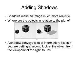
Adding Shadows. Shadows make an image much more realistic. Where are the objects in relation to the plane? A shadow conveys a lot of information; it’s as if you are getting a second look at the object from the viewpoint of the light source. Adding Shadows (2).

Adding Shadows
E N D
Presentation Transcript
Adding Shadows • Shadows make an image much more realistic. • Where are the objects in relation to the plane? • A shadow conveys a lot of information; it’s as if you are getting a second look at the object from the viewpoint of the light source.
Adding Shadows (2) • We will look at 3 methods for generating shadows. • The tools we develop will be useful only for generating shadows cast by a point light source onto a flat surface. • In Chapter 12, ray tracing tools will allow us to show accurate shadow shapes for any light source shining on any surface shape.
Shadows as Texture • The problem is to compute the shape of the shadow that is cast. • The shape of the shadow is determined by the projections of each of the faces of the box onto the plane of the floor using the source as the center of projection. The shadow is the union of the projections of the six faces.
Shadows as Texture (2) • After drawing the plane using ambient, diffuse, and specular light contributions, draw the six projections of the box’s faces on the plane using only ambient light. • This will draw the shadow in the right shape and color. • Finally draw the box. (If the box is near the plane parts of it might obscure portions of the shadow.)
Shadows as Texture • The projection of a vertex V on the original object is given by V1 = S + (V - S) ([n·(A - S)]/[n·(V - S)]), where S is the position of the light source, A is a point on the plane, and n is the normal to the plane.
Building Projected Faces • To make the new face F’ produced by F, project each of its vertices onto the plane in question. • Suppose that the plane passes through point A and has normal vector n. Consider projecting vertex V, producing point V’. Point V’ is the point where the ray from the source at S through V hits the plane. As developed in the exercises, this point is: • The exercises show how this can be written in homogeneous coordinates as V times a matrix, which is useful for rendering engines, like OpenGL, that support convenient matrix multiplication.
Shadows Using a Shadow Buffer • This method works for non-planar surfaces. • The general idea is that any point hidden from the light source is in shadow. • A second depth buffer (the shadow buffer) is used. It contains depth information about the scene from the point of view of the light source.
Shadow Buffer Steps • 1). Shadow buffer loading. The shadow buffer is first initialized with 1.0 in each element, the largest pseudodepth possible. • Then, using a camera positioned at the light source, each of the faces in the scene is scan converted, but only the pseudodepth of the point on the face is tested. • Each element of the shadow buffer keeps track of the smallest pseudodepth seen so far.
Shadow Buffer Steps (2) • Example: Suppose point P is on the ray from the source through shadow buffer “pixel” d[i][j], and that point B on the pyramid is also on this ray. If the pyramid is present, d[i][j] contains the pseudodepth to B; if it happens to be absent, d[i][j] contains the pseudodepth to P.
Shadow Buffer Steps (3) • The shadow buffer calculation is independent of the eye position. • In an animation where only the eye moves, the shadow buffer is loaded only once. • The shadow buffer must be recalculated; however, whenever the objects move relative to the light source.
Shadow Buffer Steps (4) • Render the scene. Each face in the scene is rendered using the eye camera as usual. • Suppose the eye camera sees point P through pixel p[c][r]. When rendering p[c][r] we must find • the pseudodepth D from the source to P; • the index location [i][j] in the shadow buffer that is to be tested; • the value d[i][j] stored in the shadow buffer. • If d[i][j] is less than D, the point P is in shadow, and p[c][r] is set using only ambient light. • Otherwise P is not in shadow and p[c][r] is set using ambient, diffuse, and specular light.
Shadows Using Radiosity Method (Overview) • Recall that the inclusion of ambient light in the calculation of the light components that reflect from each face of an object is a “catch-all”. Ambient is a concocted light attribute and does not exist in real life. • It attempts to summarize the many beams of light that make multiple reflections off the various surfaces in a scene. • Radiosity is a model that attempts to improve image realism. • It attempts to form an accurate model of the amount of light energy arriving at each surface versus the amount of light leaving that surface.
Radiosity Method (Overview) • The figure shows an example of radiosity: part a shows the scene using radiosity; part b shows it without radiosity. • Using radiosity increases dramatically the computational time required to render an image.
Radiosity Method (3) • Neither scene produces a high level of realism. • We will see in Ch. 12 that the use of ray tracing raises the level of realism dramatically and permits a number of specific effects (including realistic shadows) to be included.
OpenGL 2.0 and the Shading Language GLSL • Extensions allow changes and improvements to be made to OpenGL. • Extensions are created and specified by companies who wish to test and implement innovations in OpenGL, such as new sets of algorithms, functions, and access to the latest hardware capabilities.
GLSL (2) • Programmable Shading was an extension which provided the application programmer with function calls directly to the graphics card. • In OpenGL 2.0 the programmable shading extension was promoted to the core of OpenGL. • The addition of these new function calls allowed the application programmer to control shading operations directly, avoiding the fixed pipeline shading functions. • Some of the most difficult shading approaches are bump-mapping and 3D textures; the OpenGL Shading Language (GLSL) removes much of the burden of accomplishing these from the application programmer.
OpenGL Pipeline with GLSL • The figure is a simplified version of the OpenGL pipeline with the addition of the GLSL. • The pipeline begins with a collection of polygons (vertices) as input, followed by a vertex processor which runs vertex shaders.
OpenGL Pipeline with GLSL (2) • Vertex shaders are pieces of code which take vertex data as input; the data includes position, color, normals, etc. With a vertex shader an application program can perform tasks such as: • vertex position transformations; controlled by the modelview and projection matrices; • transforming the normal vectors and normalizing them if appropriate; • generating and transforming texture coordinates; • applying a light model-per-vertex (ambient, diffuse, and specular), and computing color.
OpenGL Pipeline with GLSL (3) • Once the vertices have been transformed into the viewplane, primitives are rasterized and fragments are formed. • For instance, a primitive such as a point might cover a single pixel on the screen, or a line might cover five pixels on a screen. • The fragment resulting from the point consists of a window’s coordinate and depth information, as well as other associated attributes including color, texture coordinates, depth, and so forth.
OpenGL Pipeline with GLSL (4) • Rasterization also determines the pixel position of the fragment. The values for each such attribute are found by interpolating between the values encountered at the vertices. • A line primitive that stretches across five pixels results in five fragments and the attributes of these fragments are found by interpolating between the corresponding values at the end-points of the line. • Some primitives don’t yield any fragments at all, whereas others generate a large number of fragments. • The output of the “rasterization” stage is a flow of fragments (the pipeline here is actually a suggestion to how OpenGL operates).
At each point, the texture perturbs the normal vector to the surface and consequently perturbs the normal direction that is so used to calculate each specular highlight. Bump Mapping • Bump mapping is a highly effective method for adding complex texture to objects, without having to alter their underlying geometry. • For example, this figure shows a close-up view of an orange with a rough pitted surface. However, the actually geometry of the orange is a smooth sphere and the texture has been painted on it.
Bump Mapping (2) • It is important to note that the geometry of the object is still a simple sphere, whereas the perturbing texture can be an image or other source of randomized texture as we have discussed previously. • Another example, where the surface appears to have been engraved with the dates, “1914 – 1918”. However, the indentations of the engraving are created by perturbing the normal vector.
Bump Mapping (3) • How is bump mapping done? Given an initial perturbation map with which we wish to perturb the surface normal of an object, we must calculate its effect pixel by pixel on the actual surface normal. • The derivation of this normal perturbation requires the repeated use of partial derivatives and cross-products between them. • The calculations are beyond the scope of this book. Fortunately, certain extensions to OpenGL offer some assistance in bump mapping which save the application programmer from having to use the underlying mathematics (partial derivatives, etc).
Bump Mapping (4) • There is also an excellent tutorial on this subject by Paul Baker at www.paulsprojects.net. • The figure shows an example of a torus with and without bump mapping that he develops carefully in the tutorial.
Non-Photorealistic Rendering • There are situations when realism is not the most desirable attribute of an image. • Instead one might want to emphasize a particular message in an image or omit details that are expensive to render yet of little interest to the intended audience.
Non-Photorealistic Rendering (2) • For example, one might want to produce a cartoon-like rendering of an engine as shown in the figure. This image gives the impression that it could have been done by hand with a paintbrush.
Non-Photorealistic Rendering (3) • In another situation, one might want to generate a highly-detailed and precise technical drawing of some machine or a blueprint without regard to the fineries of shading, shadows, and anti-aliasing. • This technique has been called pen and ink rendering (or engraving).
Non-Photorealistic Rendering (4) • Another example of non-photorealistic rendering; note that this image is very suggestive of what it represents even though it clearly does not look like an actual photograph of the object.