Download
1 / 29
290 likes | 418 Vues
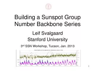
Building a Sunspot Group Number Backbone Series. Leif Svalgaard Stanford University 3 rd SSN Workshop, Tucson, Jan. 2013. Why a Backbone? And What is it?. Building a long time series from observations made over time by several observers can be done in two ways:.

E N D
Building a Sunspot Group Number Backbone Series Leif Svalgaard Stanford University 3rd SSN Workshop, Tucson, Jan. 2013
Why a Backbone? And What is it? Building a long time series from observations made over time by several observers can be done in two ways: • Daisy-chaining: successively joining observers to the ‘end’ of the series, based on overlap with the series as it extends so far [accumulates errors] • Back-boning: find a primary observer for a certain [long] interval and normalize all other observers individually to the primary based on overlap with only the primary [no accumulation of errors] Chinese Whispers When several backbones have been constructed we can join [daisy-chain] the backbones. Each backbone can be improved individually without impacting other backbones Carbon Backbone
The Backbones • SIDC Backbone [????-2013] • Japanese Backbone [1921-1995] • Wolfer Backbone [1841-1945] • Schwabe Backbone [1794-1883] • Staudach Backbone [????-????] • Earlier Backbone(s) [1610-????]
Sources of Data • The primary source is the very valuable tabulations by Hoyt and Schatten of the ‘raw’ count of groups by several hundred observers • In some cases [especially Wolf and Schwabe] data has been re-entered and re-checked from Wolf’s published lists, as some discrepancies have been found with the H&S list
The Wolfer Backbone Alfred Wolfer observed 1876-1928 with the ‘standard’ 80 mm telescope Rudolf Wolf from 1860 on mainly used smaller 37 mm telescope(s) so those observations are used for the Wolfer Backbone 37 mm X20 80 mm X64
Normalization Procedure, I What we do not do: • Compare only days when both observers actually observed. This is problematic when observations are sparse as during the early years. • Compare only days when both observers actually recorded at least one group. This is clearly wrong as it will bias towards higher activity. What we do: • We compute, for each observer, the monthly mean of actual observations [including days when it was indeed observed that there were no groups]. • We compute, for each observer and for each year, the yearly mean of the average counts for months with at least one observation.
Normalization Procedure, II F = 1202 For each Backbone we regress each observers group counts for each year against those of the primary observer, and plot the result [left panel]. Experience shows that the regression line almost always very nearly goes through the origin, so we force it to do that and calculate the slope and various statistics, such as 1-σ uncertainty and the F-value. The slope gives us what factor to multiply the observer’s count by to match the primary’s. The right panel shows a result for the Wolfer Backbone: blue is Wolf’s count [with his small telescope], pink is Wolfer’s count [with the larger telescope], and the orange curve is the blue curve multiplied by the slope. It is clear that the harmonization works well [at least for Wolf vs. Wolfer].
Schmidt, Winkler F = 2062 F = 1241
Weber, Spörer F = 2062 F = 109 F = 1241 F = 347
Tacchini, Quimby F = 2062 F = 1379 F = 1352
Broger, Leppig F = 3003 F = 953
Konkoly, Mt. Holyoke F = 2225 F = 953 Etc… Dawson, Guillaume, Bernaerts, Woinoff, Merino, Ricco, Moncalieri, Sykora, Brunner,…
The Wolfer Group Backbone Weighted by F-value If we average without weighting by the F-value we get very nearly the same result as the overlay at the left shows
Hoyt & Schatten used the Group Count from RGO [Royal Greenwich Observatory] as their Normalization Backbone. Why don’t we? Because there are strong indications that the RGO data is drifting before ~1900 Could this be caused by Wolfer’s count drifting? His k-factor for RZwas, in fact, declining slightly the first several years as assistant (seeing fewer spots early on – wrong direction). The group count is less sensitive than the Spot count and there are also the other observers… José Vaquero found a similar result which he reported at the 2nd Workshop in Brussels. Sarychev & Roshchina report in Solar Sys. Res. 2009, 43: “There is evidence that the Greenwich values obtained before 1880 and the Hoyt–Schatten series of Rg before 1908 are incorrect”.
The Schwabe Backbone Schwabe received a 50 mm telescope from Fraunhofer in 1826 Jan 22. This telescope was used for the vast majority of full-disk drawings made 1826–1867. For this backbone we use Wolf’s observations with the large 80mm standard telescope ? Schwabe’s House
Wolf, Shea Mixing records! F = 493
Schmidt, Carrington F = 161 F = 431
Spörer, Peters F = 159 F = 73
Pastorff, Weber F = 158 F = 234
Hussey, Stark’ F = 116 F = 289
Tevel, Arago F = 2.3 F = 8.3
Flaugergues, Herschel F = 0.1 F = 2.3 Etc… Lindener, Schwarzenbrunner, Derfflinger…
The Schwabe Group Backbone Weighted by F-value
Joining two Backbones Comparing Schwabe with Wolfer backbones over 1860-1883 we find a normalizing factor of 1.55 1.55
How do we Know HMF B? The IDV-index is the unsigned difference from one day to the next of the Horizontal Component of the geomagnetic field averaged over stations and a suitable time window. The index correlates strongly with HMF B [and not with solar wind speed]