Download
1 / 28
280 likes | 300 Vues
Learn how to find derivatives using Constant, Power, and Multiple Rules. Practice Sum and Difference Rules and discover how to find rates of change. Understand how derivatives are utilized to determine motion and velocity.

E N D
MATH 1910 Chapter 2 Section 2 Basic Differentiation Rules and Rates of Change
Objectives • Find the derivative of a function using the Constant Rule. • Find the derivative of a function using the Power Rule. • Find the derivative of a function using the Constant Multiple Rule.
Objectives • Find the derivative of a function using the Sum and Difference Rules. • Find the derivatives of the sine function and of the cosine function. • Use derivatives to find rates of change.
The Constant Rule Figure 2.14
The Power Rule Before proving the next rule, it is important to review the procedure for expanding a binomial. The general binomial expansion for a positive integer n is This binomial expansion is used in proving a special case of the Power Rule.
The Power Rule When using the Power Rule, the case for which n = 1 is best thought of as a separate differentiation rule. That is, This rule is consistent with the fact that the slope of the line y = x is 1, as shown in Figure 2.15. Figure 2.15
Example 2 – Using the Power Rule In Example 2(c), note that before differentiating, 1/x2 was rewritten as x-2. Rewriting is the first step in many differentiation problems.
The Constant Multiple Rule The Constant Multiple Rule and the Power Rule can be combined into one rule. The combination rule is
Rates of Change You have seen how the derivative is used to determine slope. The derivative can also be used to determine the rate of change of one variable with respect to another. Applications involving rates of change occur in a wide variety of fields. A few examples are population growth rates, production rates, water flow rates, velocity, and acceleration.
Rates of Change A common use for rate of change is to describe the motion of an object moving in a straight line. In such problems, it is customary to use either a horizontal or a vertical line with a designated origin to represent the line of motion. On such lines, movement to the right (or upward) is considered to be in the positive direction, and movement to the left (or downward) is considered to be in the negative direction.
Rates of Change The function s that gives the position (relative to the origin) of an object as a function of time t is called a position function. If, over a period of time t, the object changes its position by the amount s = s(t + t) – s(t), then, by the familiar formula the average velocity is
Example 9 –Finding Average Velocity of a Falling Object A billiard ball is dropped from a height of 100 feet. The ball’s height s at time t is the position function s = –16t2 + 100 Position function where s is measured in feet and t is measured in seconds. Find the average velocity over each of the following time intervals. a. [1, 2] b. [1, 1.5] c. [1, 1.1]
Example 9(a) –Solution For the interval [1, 2], the object falls from a height of s(1) = –16(1)2 + 100 = 84 feet to a height of s(2) = –16(2)2 +100 = 36 feet. The average velocity is
Example 9(b) –Solution cont’d For the interval [1, 1.5], the object falls from a height of 84 feet to a height of s(1.5) = –16(1.5)2 +100 = 64 feet. The average velocity is
Example 9(c) –Solution cont’d For the interval [1, 1.1], the object falls from a height of 84 feet to a height of s(1.1) = –16(1.1)2 +100 = 80.64 feet. The average velocity is Note that the average velocities are negative, indicating that the object is moving downward.
Rates of Change In general, if s = s(t) is the position function for an object moving along a straight line, the velocity of the object at time t is In other words, the velocity function is the derivative of the position function. Velocity can be negative, zero, or positive. The speed of an object is the absolute value of its velocity. Speed cannot be negative.
Rates of Change The position of a free-falling object (neglecting air resistance) under the influence of gravity can be represented by the equation where s0 is the initial height of the object, v0 is the initial velocity of the object, and g is the acceleration due to gravity. On Earth, the value of g is approximately –32 feet per second per second or –9.8 meters per second per second.
Example 10 –Using the Derivative to Find Velocity At time t = 0, a diver jumps from a platform diving board that is 32 feet above the water (see Figure 2.21). Because the initial Velocity of the diver is 16 feet per second, the position of the diver is s(t) = –16t2 + 16t + 32 Position function where s is measured in feet and t is measured in seconds. • When does the diver hit the water? b.What is the diver’s velocity at impact? Figure 2.21
Example 10(a) –Solution To find the time t when the diver hits the water, let s = 0 and solve for t. –16t2 + 16t + 32 = 0 Set position function equal to 0. –16(t + 1)(t – 2) = 0 Factor. t = –1 or 2 Solve for t. Because t≥ 0, choose the positive value to conclude that the diver hits the water at t = 2 seconds.
Example 10(b) –Solution cont’d The velocity at time t is given by the derivative s(t) = –32t + 16. So, the velocity at time is t = 2 is s(2) = –32(2) + 16 = –48 feet per second.