Gravitational Wave Detection Using Pulsar Timing Current Status and Future Progress
Gravitational Wave Detection Using Pulsar Timing Current Status and Future Progress. Fredrick A. Jenet Center for Gravitational Wave Astronomy University of Texas at Brownsville. Dick Manchester ATNF/CSIRO Australia. George Hobbs ATNF/CSIRO Australia. KJ Lee Peking U. China.

Gravitational Wave Detection Using Pulsar Timing Current Status and Future Progress
E N D
Presentation Transcript
Gravitational Wave Detection Using Pulsar TimingCurrent Status and Future Progress Fredrick A. Jenet Center for Gravitational Wave Astronomy University of Texas at Brownsville
Dick Manchester ATNF/CSIRO Australia George Hobbs ATNF/CSIRO Australia KJ Lee Peking U. China Andrea Lommen Franklin & Marshall USA Shane L. Larson Penn State USA Linqing Wen AEI Germany Collaborators John Armstrong JPL USA Teviet Creighton Caltech USA
Main Points • Radio pulsar can directly detect gravitational waves • How can you do that? • What can we learn? • Astrophysics • Gravity • Current State of affairs • What can the SKA do.
- ¶2 hmn /¶2 t + 2 hmn = 4p Tmn Gravitational Waves “Ripples in the fabric of space-time itself” gmn = hmn + hmn Gmn(g) = 8 p Tmn
Pulsar Timing • Pulsar timing is the act of measuring the arrival times of the individual pulses
How does one detect G-waves using Radio pulsars? Pulsar timing involves measuring the time-of arrival (TOA) of each individual pulse and then subtracting off the expected time-of-arrival given a physical model of the system. R = TOA – TOAm
Timing residuals from PSR B1855+09 From Jenet, Lommen, Larson, & Wen, ApJ , May, 2004 Data from Kaspi et al. 1994 Period =5.36 ms Orbital Period =12.32 days
1010 Msun BBH 10-12 OJ287 3C 66B * * @ a distance of 20 Mpc 10-13 109 Msun BBH @ a distance of 20 Mpc h 10-14 SMBH Background 10-15 10-16 3 10-11 3 10-10 3 10-9 3 10-8 3 10-7 Frequency, Hz Sensitivity of a Pulsar timing “Detector” h = W R Rrms 1 m s h >= 1 ms W/N1/2
The Stochastic Background Characterized by its “Characterictic Strain” Spectrum: hc(f) = A f gw(f) = (2 2/3 H02) f2 hc(f)2 Super-massive Black Holes: = -2/3 A = 10-15 - 10-14 yrs-2/3 For Cosmic Strings: = -7/6 A= 10-21 - 10-15 yrs-7/6 • Jaffe & Backer (2002) • Wyithe & Lobe (2002) • Enoki, Inoue, Nagashima, Sugiyama (2004) • Damour & Vilenkin (2005)
The Stochastic Background The best limits on the background are due to pulsar timing. For the case where gw(f) is assumed to be a constant (=-1): Kaspi et al (1994) report gwh2 < 6 10-8 (95% confidence) McHugh et al. (1996) report gwh2 < 9.3 10-8 Frequentist Analysis using Monte-Carlo simulations Yield gwh2 < 1.2 10-7
The Stochastic Background The Parkes Pulsar Timing Array Project Goal: Time 20 pulsars with 100 nano-second residual RMS over 5 years Current Status Timing 20 pulsars for 2 years, 5 currently have an RMS < 300 ns Combining this data with the Kaspi et al data yields: = -1 : A<4 10-15 yrs-1 gwh2 < 8.8 10-9 = -2/3 : A<6.5 10-15 yrs-2/3gw(1/20 yrs)h2 < 3.0 10-9 = -7/6 : A<2.2 10-15 yrs-7/6gw(1/20 yrs)h2 < 6.9 10-9
The Stochastic Background With the SKA: 40 pulsars, 10 ns RMS, 10 years = -1 : A<3.6 10-17gwh2 < 6.8 10-13 = -2/3 : A<6.0 10-17gw(1/10 yrs)h^2 < 4.0 10-13 = -7/6 : A<2.0 10-17gw(1/10 yrs)h^2 < 2.1 10-13
The Stochastic Background A Dream, or almost reality with SKA: 40 pulsars, 1 ns RMS, 20 years = -2/3 : A<1.0 10-18gw(1/10 yrs)h^2 < 1.0 10-16 The expected background due to white dwarf binaries lies in the range of A = 10-18 - 10-17! (Phinney (2001)) • Individual 108 solar mass black hole binaries out to ~100 Mpc. • Individual 109 solar mass black hole binaries out to ~1 Gpc
The timing residuals for a stochastic background This is the same for all pulsars. This depends on the pulsar. The induced residuals for different pulsars will be correlated.
The Expected Correlation Function Assuming the G-wave background is isotropic:
How to detect the Background For a set of Np pulsars, calculate all the possible correlations:
How to detect the Background Search for the presence of h(q) in C(q):
How to detect the Background The expected value of r is given by: In the absence of a correlation, r will be Gaussianly distributed with:
How to detect the Background The significance of a measured correlation is given by:
For a background of SMBH binaries: hc = A f-2/3 20 pulsars. Single Pulsar Limit (1 ms, 7 years) Expected Regime
For a background of SMBH binaries: hc = A f-2/3 20 pulsars. Single Pulsar Limit (1 ms, 7 years) Expected Regime 1 ms, 1 year
For a background of SMBH binaries: hc = A f-2/3 20 pulsars. Single Pulsar Limit (1 ms, 7 years) Expected Regime 1 ms, 1 year (Current ability) .1 m s 5 years
For a background of SMBH binaries: hc = A f-2/3 20 pulsars. Single Pulsar Limit (1 ms, 7 years) Expected Regime 1 ms, 1 year (Current ability) .1 s 10 years .1 m s 5 years
Single Pulsar Limit (1 ms, 7 years) Expected Regime 1 ms, 1 year (Current ability) Detection SNR for a given level of the SMBH background Using 20 pulsars hc = A f-2/3 SKA 10 ns 5 years 40 pulsars .1 s 10 years .1 m s 5 years
Graviton Mass • Current solar system limits place mg < 4.4 10-22 eV • 2 = k2 + (2 mg/h)2 • c = 1/ (4 months) • Detecting 5 year period G-waves reduces the upper bound on the graviton mass by a factor of 15. • By comparing E&M and G-wave measurements, LISA is expected to make a 3-5 times improvement using LMXRB’s and perhaps up to 10 times better using Helium Cataclismic Variables. (Cutler et al. 2002)
Radio pulsars can directly detect gravitational waves • R = h/s , 100 ns (current), 10 ns (SKA) • What can we learn? • Is GR correct? • SKA will allow a high SNR measurement of the residual correlation function -> Test polarization properties of G-waves • Detection implies best limit of Graviton Mass (15-30 x) • The spectrum of the background set by the astrophysics of the source. • For SMBHs : Rate, Mass, Distribution (Help LISA?) • Current Limits • For SMBH, A<6.5 10-15 or gw(1/20 yrs)h2 < 3.0 10-9 • SKA Limits • For SMBH, A<6.0 10-17 or gw(1/10 yrs)h2 < 4.0 10-13 • Dreamland: A<1.0 10-18 or gw(1/10 yrs)h2 < 1.0 10-16 • Individual 108 solar mass black hole binaries out to ~100 Mpc. • Individual 109 solar mass black hole binaries out to ~1 Gpc