Hough Transform
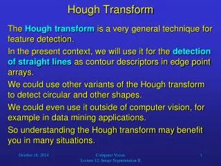
Hough Transform. The Hough transform is a very general technique for feature detection. In the present context, we will use it for the detection of straight lines as contour descriptors in edge point arrays.

Hough Transform
E N D
Presentation Transcript
Hough Transform • The Hough transform is a very general technique for feature detection. • In the present context, we will use it for the detection of straight lines as contour descriptors in edge point arrays. • We could use other variants of the Hough transform to detect circular and other shapes. • We could even use it outside of computer vision, for example in data mining applications. • So understanding the Hough transform may benefit you in many situations. Computer Vision Lecture 12: Image Segmentation II
Hough Transform • The Hough transform is a voting mechanism. • In general, each point in the input space votes for several combinations of parameters in the output space. • Those combinations of parameters that receive the most votes are declared the winners. • We will use the Hough transform to fit a straight line to edge position data. • To keep the description simple and consistent, let us assume that the input image is continuous and described by an x-y coordinate system. Computer Vision Lecture 12: Image Segmentation II
Hough Transform • A straight line can be described by the equation: • y = mx + c • The variables x and y are the parameters of our input space, and m and c are the parameters of the output space. • For a given value (x, y) indicating the position of an edge in the input, we can determine the possible values of m and c by rewriting the above equation: • c = -xm + y • You see that this represents a straight line in m-c space, which is our output space. Computer Vision Lecture 12: Image Segmentation II
y c C C winner parameters B B A A 0 x 0 m input space output space Hough Transform • Example: Each of the three points A, B, and C on a straight line in input space are transformed into straight lines in output space. The parameters of their crossing point (which would be the winners) are the parameters of the straight line in input space. Computer Vision Lecture 12: Image Segmentation II
Hough Transform • Hough Transform Algorithm: • Quantize input and output spaces appropriately. • Assume that each cell in the parameter (output) space is an accumulator (counter). Initialize all cells to zero. • For each point (x, y) in the image (input) space, increment by one each of the accumulators that satisfy the equation. • Maxima in the accumulator array correspond to the parameters of model instances. Computer Vision Lecture 12: Image Segmentation II
Hough Transform • The Hough transform does not require preprocessing of edge information such as ordering, noise removal, or filling of gaps. • It simply provides an estimate of how to best fit a straight line (or other curve model) to the available edge data. • If there are multiple straight lines in the image, the Hough transform will result in multiple peaks. You can search for these peaks to find the parameters for all the corresponding straight lines. Computer Vision Lecture 12: Image Segmentation II
Improved Hough Transform • Here is some practical advice for doing the Hough transform (e.g., for some future assignment). • The m-c space described on the previous slides is simple but not very practical. It cannot represent vertical lines, and the closer the orientation of a line gets to being vertical, the greater is the change in m required to turn the line significantly. • We are going to discuss an alternative output space that requires a bit more computation but avoids the problems of the m-c space. Computer Vision Lecture 12: Image Segmentation II
Improved Hough Transform • As we said before, it is problematic to use m (slope) and c (intercept) as an output space. • Instead, it is a good idea to use the orientation and length d of the normal of a straight line to describe it. • The normal n of a straight line l is perpendicular to l and connects l with the origin of the coordinate system. • The range of is from 0 to 360, and the range of d is from 0 to the length of the image diagonal. • Note that we can skip the interval from 180 to 270, because it would require a negative d. • Let us assume that the image is 450×450 units large. Computer Vision Lecture 12: Image Segmentation II
636 representation of same line in output space line to be described d d 0 0 360 output space Improved Hough Transform Column j 0 450 0 Row i 450 input space The parameters and d form the output space for our Hough transform. Computer Vision Lecture 12: Image Segmentation II
Improved Hough Transform • For any edge point (i0, j0) indicated by our Sobel edge detector, we have to find all parameters and d for those straight lines that pass through (i0, j0). • We will then increase the counters in our output space located at every (, d) by the edge strength, i.e., the magnitude provided by the Sobel detector. • This way we will find out which parameters (, d) are most likely to indicate the clearest lines in the image. • But first of all, we have to discuss how to find all the parameters (, d) for a given point (i0, j0). Computer Vision Lecture 12: Image Segmentation II
450 (i0, j0) Column j d2 d1 2 d3 0 1 3 0 450 Row i Improved Hough Transform By varying from 0 to 360 we can find all lines crossing (i0, j0): But how can we compute parameter d for each value of ? Idea: Rotate (i0, j0) around origin by - so that it lands on i-axis. Then the i-coordinate of the rotated point is the value of d. Computer Vision Lecture 12: Image Segmentation II
Improved Hough Transform • And how do we rotate a point in two-dimensional space? • The simplest way is to multiply the point vector with a rotation matrix. • We compute the rotated point (iR, jR) as obtained by rotation of point (i0, j0) around the point (0, 0) by the angle as follows: Computer Vision Lecture 12: Image Segmentation II
Improved Hough Transform • We are only interested in the i-coordinate: • iR= i0 cos - j0 sin • In our case, we want to rotate by the angle -: • iR= i0 cos(-) - j0 sin(-) • iR= i0 cos + j0 sin • Now we can compute parameter d as a function of i0, j0, and : • d(i0, j0;) = i0 cos + j0 sin • By varying we are now able to determine all parameters (, d) for a given point (i0, j0) and increase the counters in output space accordingly. Computer Vision Lecture 12: Image Segmentation II
Improved Hough Transform • We can then define the straight line representing the “winner” in parametric form using a parameter p. • The points (i, j) of the line are then given by the following equation: By varying p within an appropriate range, we can compute every pixel of our straight line. But how can we find the vector (i, j) that determines the slope of the line? Computer Vision Lecture 12: Image Segmentation II
Improved Hough Transform • The idea here is that the orientation of the straight line is perpendicular to its normal. • Since the orientation of the normal is given by the angle , the orientation of the straight line must be given by - 90. • Therefore, we get: Computer Vision Lecture 12: Image Segmentation II
Improved Hough Transform • Then the complete equation for the straight line with parameters (, d) looks like this: Just vary parameter p in steps of 1 (to catch every pixel) between approximately -900 to 900 (twice the image size). Whenever (i, j) is within the image range, then visualize that pixel in the bitmap. Computer Vision Lecture 12: Image Segmentation II
Sample Results • Input Image Computer Vision Lecture 12: Image Segmentation II
Sample Results • Edges in input image (Sobel filter output) Computer Vision Lecture 12: Image Segmentation II
Sample Results • d • -90 • Hough-transformed edge image • 0 • • 90 • 180 Computer Vision Lecture 12: Image Segmentation II
Sample Results • d • 270 • Five greatest maxima in Hough-transformed image • 0 • • 90 • 180 Computer Vision Lecture 12: Image Segmentation II
Sample Results • Lines in input image corresponding to Hough maxima Computer Vision Lecture 12: Image Segmentation II