Download
1 / 23
230 likes | 251 Vues
This workshop outlines the Hough Transform (HT) approach for fast filling of Hough space to track particle trajectories. Results include efficiency, fake reduction, resolution, and time consumption considerations. The method is shown to overcome problems in high multiplicity events and offers fast tracking with low fake track rates. Recent developments aim to enhance speed and add online PID capabilities. The HT method transforms TPC digit coordinates into track parameter space, guiding track extraction through peak finding over the Hough space. Linearly filling the Hough space variables accelerates track identification. The workshop details recent improvements for code speed-up while maintaining algorithm efficiency.

E N D
Status of Hough Transform TPC Tracker C.Cheshkov
Outline • Introduction • Hough Transform (HT) approach: • Description of the algorithm • Practical implementation for fast filling of the Hough space • Hough space variables • Recent improvements • Results: • Efficiency, fakes • Resolution • Time consumption (!) • Conclusions & Plans HLT workshop
Introduction • It has been already shown that the presented HT method: • Overcomes the common problems in high multiplicity PbPb events • Provides reasonably high tracking efficiency and low fake tracks rate • Can work not only as a seeding for consecutive cluster finder/fitter, but also as a stand-alone tracking algorithm • Extremely fast • The recent developments were oriented towards: • Further speeding up To be able to track central PbPb events online, by means of purely software version of HT • AddingdEdxreconstruction online PID • Studies of the sources of inefficiencies and fakes HLT workshop
Hough Transform method • Hough Transform method: • Transformation of TPC Digit coordinates into curve in the track parameter space (Hough space). The curve corresponds to all possible tracks the digit can belong to • The transformation is done in bins • Assume that the tracks are coming from the primary vertex • Neglect multiply scattering and energy losses • Each space bin represents a track candidate one can define a certain “road” within a given TPC sector • The approach consists simply in counting of the number of TPC rows without a digit inside the track “road” - #gaps HLT workshop
Hough Transform method • After the HT is finished, a simple peak finder runs over the Hough space in order to extract the track candidates • The peak finder looks for neighbor bins with #gaps<N and identifies the peaks(track candidates) • Track parameters are extracted by averaging the peak edge points track is guided by the cluster borders HLT workshop
Hough Transform method • Assuming ordered TPC digits (in time bins, pads, padrows) the algorithm offers big space for speeding up! • HT is monotonic along the padrows do it only for the first and last (in pad index direction) digits which belong to a cluster and fill at once the corresponding ribbon in the HT space • Stopping rule using already accumulated #gaps HLT workshop
Hough Space variables • Initially Hough space defined by track curvature k(=1/R) and emission angle • Two main problems: • The variables are strongly correlated “Butterfly”-like shape of the peaks • complex peak finder • relatively high fake peak rate • Non-linear functions in the filling of HT space • Need in LUTs inside HT filling loop • “Time consuming” FP operations inside HT filling loop • Better solution was found HLT workshop
Lets define two curves inside a TPC sector by x/R2 = constant = 1(2) Each primary track is represented by two points on these curves One can parameterize the track using: 1=y1/R12 and 2=y2/R22 Conformal map coordinates of each space-point along the track trajectory are connected by linear expression Conformal Map transformation variables were chosen: Variables connected to the physical setup of the TPC Variables which lead to linear HT (x1,y1) (x2,y2) Hough Space variables TPC sector layout HLT workshop
Hough Space variables • One can use the variables 1 and 2 to define the Hough space • In this way each space-point inside a TPC sector will be represented in the Hough space by a straight line: 1 = A + B 2 Linear filling of the Hough space • The parameters A and B are calculated in advance and used via LUTs • In order to keep HT monotonic and Hough peaks uncorrelated: curve 1 – in middle and curve 2 – at the outer edge of the TPC sector HLT workshop
Example slice of TPC sector Corresponding Hough Space • Uncorrelated and easily detectable Hough peaks • Linear HT Gain of 30-40% in the time consumption HLT workshop
Hough Space variables • Limits on Hough space variables correspond to a track with minimum Pt[GeV/c] = Bfield[T] which crosses the middle of the TPC sector • Hough space binning is fixed to ~ twice the pad size in the corresponding TPC rows 80(1)x120(2)x100() HLT workshop
Recent improvements • All the recent changes are aimed to speed up the code and do not affect the algorithm efficiency • There are no revolutionary improvement – all the changes give an effect of 30-50% • The overall speed-up factor is ~3 HLT workshop
Recent improvements • Change in the order in which the readout patches are processed • Choose an order which allows the earliest possible removal of track candidates (Hough space bins) • Why patches 6 and 3 before others? Digits in patch 6 – horizontal lines in the Hough Space, in patch 3 – vertical lines the crossings of these lines gives sort of seeding Old New 6 6 5 5 TPC sector 4 4 3 3 2 2 1 1 HLT workshop
Recent improvements • Selective filling of the Hough space: • For each bin of the hough space assign pointers to the closest possible track candidate (bin) • Update the pointers after each processed readout patch • Use the pointers to jump in the hough space during the filling process • Floating operations used to calculate the cluster properties in the hough space pre-calculated LUTs • Conformal mapper variables as a hough space variables • Therefore a TPC cluster is represented by 2 straight lines: 2 offsets and 2 slopes HLT workshop
Results: Efficiency, resolution and timings HLT workshop
Definitions • The method requires new definitions in order to determine the performance: • No clusters associated assign only 1 MC label to each track • High occupancy (and therefore overlapping clusters) in general does not affect the track parameters, but cause appearance of “ghosts” fakes tracks ghost tracks • If more than 1 track with the same MC label, take randomly one as good and second as fake (or ghost) • Good tracks – from offline comparison macro HLT workshop
Tracking Efficiency dN/dy=8000 dN/dy=6000 dN/dy=4000 dN/dy=2000 B=0.5T HLT workshop
Inefficiency Sources • Merging of the tracks (1-2% for dN/dy=8000, 0.4T) when: • they overlap in the hough space • they are close to each other and one is removed during the track merging (both in hough space and bins) • Low pt tracks at high (->1). • The bins efficiently get narrower • Mult.scat. in ITS & dead zone • binning (during binning we assume straight tracks) • Tracks close to the TPC sector borders (affects mainly tracks with Pt>1-1.5GeV/c) HLT workshop
Inefficiency Sources Low Pt tracks Tracks with 1.5<Pt<2 GeV/c HLT workshop
Ghost Tracks dN/dy=8000, 0.5T • Tracks found in 2 slices or 2 neighbor sectors can be further suppressed by more complex track merging procedure • However ITS tracking “removes” almost completely these ghosts no real need in further merging In 2 slices In 2 TPC sectors Overall HLT workshop
Resolution • Since the Hough space bin size ~1/Pt Pt/Pt ~ Pt + const.(mult.scat.) • Pt/Pt=(1.8xPt+1.0)% (B=0.5T) • ()=6.1mad; ()=5.5x10⁻³ • No significant dependency on the event multiplicity can be seen – need more statistics HLT workshop
Timing performance • The benchmarks were done on Itanium II machines (~1300 SpecInt’s) – the present Alice GDCs • Code compiled with icc8.0 with –O3 • Almost a factor of 3 improvement due to the latest improvements in the filling of the Hough space • LUT initialization is done of event-by-event basis more flexibility if one wants to adapt the HT resolution depending on the trigger HLT workshop
Conclusion and Outlook • Hough Transform tracker shows very good efficiency and resolution (see also Constantin’s transparencies on jet analysis) • Taking into account the presented timing performance, one should consider seriously HT as a possible online tracking for HLT (details in my talk on online monitoring) • The work on adding dEdx reconstruction is underway (see tomorrow’s talk) • Important feedback expected from the physics analysis of PDC’04 data • The algorithm (together with HLT ITS tracker) will be tested in close to real conditions during the Alice computing DC in 2005 HLT workshop