Download
1 / 58
590 likes | 807 Vues
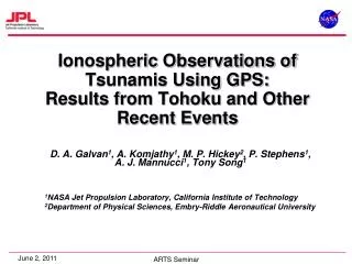
Ionospheric Observations of Tsunamis Using GPS: Results from Tohoku and Other Recent Events. D. A. Galvan 1 , A. Komjathy 1 , M. P. Hickey 2 , P. Stephens 1 , A. J. Mannucci 1 , Tony Song 1 1 NASA Jet Propulsion Laboratory, California Institute of Technology

E N D
Ionospheric Observations of Tsunamis Using GPS: Results from Tohoku and Other Recent Events D. A. Galvan1, A. Komjathy1, M. P. Hickey2, P. Stephens1, A. J. Mannucci1, Tony Song1 1NASA Jet Propulsion Laboratory, California Institute of Technology 2Department of Physical Sciences, Embry-Riddle Aeronautical University
Outline • Tsunami Characteristics as a Natural Hazard • Phenomenology: Ocean-Ionosphere Coupling • Total Electron Content Measurements • Observations • 2009 American Samoa Tsunami • 2010 Chile Tsunami • 2011 Tohoku Tsunami • Conclusions
1. Tsunamis as a Natural Hazard • Series of ocean waves caused by displacement of large volume of water. (Earthquakes, landslides, underwater nuclear detonations, bolide impacts) • Fast: Move through deep ocean at speeds ~200 m/s (~450 mph), amplitudes of several cm in deep ocean. • Typical period is 5 – 60 minutes, wavelengths ~ 100 - 400 km. (depending on ocean depth) • Can cause significant damage and loss of life • 2011 Japan Tsunami 15,327 deaths (8,343 missing) • 2010 Chile Tsunami 231 deaths • 2009 American Samoa Tsunami 192 deaths • 2004 Sumatra Tsunami 230,000 deaths • according to: NGDC http://www.ngdc.noaa.gov/hazard/tsu_db.shtml • And Japan National Police Agency http://www.npa.go.jp/archive/keibi/biki/higaijokyo_e.pdf
Tsunami Generation Figure from: http://www.globalsecurity.org/eye/images/tsunami-2.jpg
Tsunami Wave Characteristics Shallow water velocity equation: Where g = gravity d = depth 198 m/s 22 m/s http://www.globalsecurity.org/eye/images/tsunami-3.jpg
Present Day Early Warning System:Deep Ocean Assessment and Reporting of Tsunamis (DART) http://www.ndbc.noaa.gov/dart/dart.shtml
Present Day Early Warning System 2004: 6 Stations 2008 (and present day): 39 Stations operating http://www.ndbc.noaa.gov/dart.shtml
Motivation:Why add ionospheric observations? • DART buoy system is expensive: • ~$250,000 per buoy to build • DART system cost $12 M to maintain/operate in 2009 (28% of NOAA’s total tsunami-related budget)* • Buoys are sparsely distributed, temperamental • Data available 84% of time, outages due to harsh weather, human error* • GPS Receivers are more abundant, multi-use, low-cost • Additional means of observing tsunamis over a broader area could help to validate and improve theoretical model predictions, contributing to tsunami early warning system. *Government Accountability Office (GAO) report, April 2010 http://www.gao.gov/cgi-bin/getrpt?GAO-10-490
2. Phenomenology: Ocean-Atmosphere CouplingInternal Gravity Waves • Ocean waves produce atmospheric pressure waves large enough to perturb ionospheric electron densities ~1%. Daniels (1952). • Hines (1972) produced model of Internal Gravity Waves that can propagate to ionospheric altitudes based on surface disturbances. • Peltier and Hines (1976):Suggested that tsunamis could generate internal gravity waves that could be detected in the ionosphere using ionosondes. Figure from Hines, 1972
Atmosphere as Low-pass Filter • Brunt Vaisala Frequency: • g = gravity, θ = potential temperature. • ~5 mHz (period 3.3 min) at sea level. • Typical buoyancy frequency of the atmosphere. IE: any buoyancy wave must have lower frequency to propagate upward. • Typical ocean “noise” of 1 m amplitude has periods of several seconds. Too short. • Tsunamis have longer periods, typically 5 minutes – 30 minutes (3 mHz – 0.5 mHz) • Atmosphere acts as a low-pass filter, allowing tsunami-driven gravity waves to propagate upward. Figure from Kelley, 2009 after Yeh and Liu, 1974
Tsunami-driven Traveling Ionospheric Disturbances(TIDs) From Artru et al., 2005
Seismic Disturbances in the Atmosphere Sound speed model from Artru et al, 2005 3,400 m/s Figure from Garcia et al., 2005
3. Total Electron Content From Komjathy Ph.D. Dissertation, 1997.
Previous Observations • Artru et al., 2005a: Ionospheric perturbation observed on June 24, 2001 after an 8.2 M earthquake in Peru. The color points show the TEC variations at the ionospheric piercing points. A wave-like disturbance is propagating towards the coast of Honshu.
Previous Observations • Challenge: TIDs are common and difficult to distinguish from tsunamigenic IGWs, except by time of occurrence. Artru et al., 2005a
Modeling Neutral-Plasma Coupling Ne perturbations for Northward propagation including mean winds. Max value: 3 x 10⁹ m-3. Ne perturbations for Eastward propagation including mean winds. Max value: 109 m-3. • Strong zonal background winds affect TEC perturbation: • Tsunamis propagating East-West (perturbations ~0.02 TECU) • Tsunamis propagating North-South (perturbations ~3 TECU). (Hickey et al., 2009). Figures from Hickey et al., 2009
Modeling Neutral-Plasma Coupling • Strong zonal background winds affect TEC perturbation: • Tsunamis propagating East-West (perturbations ~0.02 TECU) • Tsunamis propagating North-South (perturbations ~3 TECU). (Hickey et al., 2009). Figures from Hickey et al., 2009
Data Type: Total Electron Content (TEC) from International GNSS System (IGS) stations -30-second TEC data from 355 active dual-frequency GPS receivers. -Data processed through Global Ionospheric Mapping (GIM) algorithm at JPL -For simultaneous bias identification/removal (satellite and receiver) ,
Regional Networks GEONET Array Source: Scripps Orbit and Permanent Array Center (SOPAC) GPS Data Archive, UCSD http://sopac.ucsd.edu/cgi-bin/somi4i Source: Japanese GPS Earth Observation Network (GEONET) Array Over 1200 stations http://terras.gsi.go.jp/gps/geonet_top.html
Streaming 1-second data availability Currently up to 130 stations worldwide providing 1-second realtime data. http://www.gdgps.net/, ftp://cddis.gsfc.nasa.gov/pub/gps/data/highrate
Methodology • Estimate time at which tsunami should arrive in a given region. (simple 200 m/s projection, MOST model predictions, etc.) • Process GPS TEC data from regional receivers using JPL Global Ionospheric Mapping software. • Fit high-order polynomial to time series; look at residuals. • Apply bi-directional band-pass filter: 0.5 – 5 mHz (33.3 – 3 min period) • Plot filtered TEC as a function of distance/time to search for possible tsunami-driven variations.
4. ObservationsTEC Observations: ASPA with GPS 40 Earthquake: 17:48 UT Tsunami observed at Pago Pago tidal gauge: 18:12 UT
American Samoa: Near Epicenter 3400 m/s Rayleigh Waves(Earthquake) 1000 m/s Acoustic Waves (Earthquake) 200 m/s Internal Gravity Waves (Tsunami)
MOST model of Tsunami Propagation:American Samoa, 2009 Movie available at: http://nctr.pmel.noaa.gov/samoa20090929/20090929_samoa_a.mov
American Samoa Tsunami 9/29/09 Observed at Hawaii Galvan et al., 2011 (JGR)
American Samoa Tsunami 9/29/09Observed at Hawaii (zoomed in)
American Samoa Tsunami 9/29/09Observed at Hawaii (hodochron plot)
MOST model of Tsunami PropagationChile 2010 Movie available at: http://nctr.pmel.noaa.gov, Courtesy NOAA CTR
Chile Event Observed at Hawaii >40 deg Elevation angle
Theoretical Model Results Ocean Surface Displacement (m) Vertical TEC Spectral full-wave model (SFWM), Hickey et al., 2009, using input wave form from Peltier and Hines, 1976, and period/velocity from DART buoy.
Hickey Model Compared with Data Filtered VTEC (TECU) Universal Time (2/28/2010)
Tohoku Tsunami 3/11/2011MOST model of Tsunami Propagation Movie available at: http://nctr.pmel.noaa.gov, Courtesy NOAA CTR
Tohoku Earthquake and Tsunami 3/11/2011Ionosphere Observations Bi-directional filter
Tohoku Earthquake and Tsunami 3/11/2011With Tony Song’s Model
TEC Observations over Japn 3/11/201130-second data Earthquake: 05:46:23 UT
Pre-quake ramp-up is a dual-pass filter artifact Earthquake: 05:46:23 UT
Pre-quake ramp-up is a dual-pass filter artifact Earthquake: 05:46:23 UT
Tohoku Earthquake and Tsunami 3/11/2011with model Single Direction Filter
Tohoku Earthquake and Tsunami 3/11/2011with model Single Direction Filter (trimmed)
Japan Tsunami 3/11/2011Distance vs. Time plot Distance from Epicenter UT Mar 11, 2011
Japan Tsunami 3/11/2011Distance vs. Time plot Distance from Epicenter UT Mar 11, 2011