Statistical Multiattribute Analysis
3D Seismic Attributes for Prospect Identification and Reservoir Characterization. Kurt J. Marfurt (The University of Oklahoma). Statistical Multiattribute Analysis. Course Outline Introduction Complex Trace, Horizon, and Formation Attributes Multiattribute Display

Statistical Multiattribute Analysis
E N D
Presentation Transcript
3D Seismic Attributes for Prospect Identification and Reservoir Characterization Kurt J. Marfurt (The University of Oklahoma) Statistical Multiattribute Analysis
Course Outline • Introduction • Complex Trace, Horizon, and Formation Attributes • Multiattribute Display • Spectral Decomposition • Geometric Attributes • Attribute Expression of Geology • Tectonic deformation • Clastic depositional environments • Carbonate deposition environments • Shallow stratigraphy and drilling hazards • Igneous and intrusive reservoirs and seals • Impact of Acquisition and Processing on Attributes • Attribute Prediction of Fractures and Stress • Data Conditioning • Inversion for Acoustic and Elastic Impedance • Image Enhancement and Object Extraction • Interactive Multiattribute Analysis • Statistical Multiattribute Analysis • Unsupervised Multiattribute Classification • Supervised Multiattribute Classification • Attributes and hydraulic fracturing of shale reservoirs • Attribute expression of the Mississippi Lime
Multiattribute Analysis Tools Interpreter-Driven Multiattribute Analysis Machine Learning Multiattribute Analysis Unsupervised Learning • K-means • Mixture Models • Kohonen Self-Organizing Maps • Generative Topographical Maps Interactive Analysis • Cross-correlation on Maps • Cross-plotting and Geobodies • Connected Component Labeling • Component Analysis • Image Grand Tour Statistical Analysis • Analysis of Variance (ANOVA, MANOVA) • Multilinear Regression • Kriging with external drift • Collocated co-kriging Supervised Learning • Statistical Pattern Recognition • Support Vector Machine • Projection Pursuit • Artificial Neural Networks
Discriminant Analysis Lithology group A Discriminant function Attribute 2 Lithology group B Attribute 1 (Bosch et al., 2002)
Discriminant analysis and prestack simultaneous inversion 9.0 9.4 8.0 ln(ZS) ln(ρ) Fluid line 9.2 Fluid line Δln(ρ) Δln(ZS) 7.0 9.0 9.6 9.6 9.8 9.8 10.0 10.0 10.2 10.2 ln(ZP) ln(ZP) (Russell et al, 2006)
Discriminant Analysis using frequency attributes (http://members.ozemail.com.au/~jollys/discrim.htm)
Discriminant Analysis using frequency attributes Class 3 Class 1 Class 2 function 1 = (Duration * 0.152) + (Max freq * -0.125) + (Avg freq * 0.272) + (End freq * 0.094) + (Start slope * -0.023) + (End slope * 0.156) + (Curve * 1.360) - 3.738 function 2 = (Duration * 0.531) + (Max freq * 0.056) + (Avg freq * -0.143) + (End freq * 0.343) + (Start slope * 0.541) + (End slope * -0.546) + (Curve * -0.348) - 9.748 (http://members.ozemail.com.au/~jollys/discrim.htm)
Embedded distributions Good separation, clustered Partial separation, clustered No separation, clustered No separation, partially clustered Good separation, unclustered Partial separation, unclustered No separation, unclustered (Michelena et al., 2011)
Embedded distributions (Michelena et al., 2011)
Embedded distributions Poorly separated lithology classification Better separated facies classification (Michelena et al., 2011)
Embedded distributions PDF using 39 wells PDF using 4 wells (Michelena et al., 2011)
Multiattribute Analysis Tools Exploratory Data Analysis A rigorous review of geostatistics Statistical Analysis • Analysis of Variance (ANOVA, MANOVA) • Multilinear Regression • Kriging with external drift • Collocated co-kriging
Why geostatistics rather than regular statistics? B A The data points of map A have: Count = 100 Average = Zavg, Standard deviation = σ Median = M 10 percentile = P10 90 percentile = P90 Amplitude High Low Map B has the same data points arranged in a different spatial distribution and so has identical statistical properties. Thus, classical statistics cannot distinguish or delineate their spatial continuity. (Courtesy Richard Lee, Marathon Oil Co.)
The Variogram A A B B Variance Variance Variogram B Variogram A Lag distance Lag distance Amplitude High Low (Courtesy Richard Lee, Marathon Oil Co.)
Variogram Z6 Z3 Z9 Z2 Z4 Z8 Z7 Z10 Z1 Z5 Z3 Z2 Z4 Z8 Z7 Z10 Z5 Z1 Z9 Z6 Lag distance The Variogram (semi-variogram) where h = lag distance = 1000 m (Courtesy Richard Lee, Marathon Oil Co.)
Variogram Z3 Z9 Z2 Z4 Z8 Z7 Z10 Z5 Z6 Z1 Z9 Z4 Z8 Z7 Z10 Z5 Z1 Z6 Z3 Z2 Lag distance The Variogram where h = lag distance = 2000 m (Courtesy Richard Lee, Marathon Oil Co.)
Variogram Z3 Z9 Z2 Z4 Z8 Z7 Z10 Z5 Z6 Z1 Z9 Z4 Z8 Z7 Z10 Z5 Z1 Z6 Z3 Z2 Lag distance The Variogram where h = lag distance = 3000 m (Courtesy Richard Lee, Marathon Oil Co.)
Model Range Sill Nugget The Variogram Variogram Lag distance Variograms are modeled mathematically to facilitate geostatistical computation (Courtesy Richard Lee, Marathon Oil Co.)
Some common variogrammodels Linear Spherical Exponential Variogram Variogram Variogram Lag distance Lag distance Lag distance (Courtesy Richard Lee, Marathon Oil Co.)
Interpolation can be performed in many ways amongst which is the weighted linear sum technique: where Zj= value at location j λj= weight at locationj Σλj= 1 N = number of data points within the maximum radius, R Z1 λ1 Z(estimate) λ3 λ2 Z3 Z2 Interpolation N = 3 (Courtesy Richard Lee, Marathon Oil Co.)
For example, the inverse distance squared method, where dj= distance of location j from the location to be estimated Interpolation Z1 N = 3 d1, λ1 Z(estimate) d2, λ2 d3, λ3 Z3 Z2 (Courtesy Richard Lee, Marathon Oil Co.)
Instead of the inverse distance, let’s use the inverse of the variance (the covariance) where dj= distance of location j from the location to be estimated Kriging Z1 N = 3 d1, λ1 Z(estimate) d2, λ2 d3, λ3 Z3 Z2 (Courtesy Richard Lee, Marathon Oil Co.)
A (hard, sparse) B (soft, dense) Correlation A B Variogram A Variogram B Variance Undersampled, poor estimate Variance Distance Distance Kriging with External Drift A data integration technique that utilizes the spatial continuity model of the secondary data (e.g. seismic horizon depth) to compute the weights for the interpolation of the primary data (e.g. well tops). (Courtesy Richard Lee, Marathon Oil Co.)
Kriging with External Drift (Dubrule, 2003)
Kriging with External Drift (Courtesy Marcelo Sanchez, Schlumberger)
A (hard, sparse) B (soft, dense) Correlation A B Variogram A Variogram B Variance Undersampled, poor estimate Variance Distance Distance Collocated Cokriging A technique that utilizes the spatial continuity models of the primary and secondary data sets as well as their correlation coefficient to compute the weights for the interpolation. Cross-Variogram A&B Variance Distance (Courtesy Richard Lee, Marathon Oil Co.)
Variogram 3 2 Adequately sampled 1 Conditional Simulation (Sequential Gaussian Simulation) • Perform normal-score transform to data to assure normal distribution Wells (Courtesy Richard Lee, Marathon Oil Co.)
Variogram 3 2 Conditioned local Cumulative Distribution Function Adequately sampled Random 1 Local neighborhood Conditional Simulation (Sequential Gaussian Simulation) • Perform normal-score transform to data to assure normal distribution Local Mean, μ1, variance, σ12 1 Wells 0 φ 0.3 0.0 (Courtesy Richard Lee, Marathon Oil Co.)
Variogram 3 2 Conditioned local Cumulative Distribution Function Adequately sampled Random Local neighborhood Conditional Simulation (Sequential Gaussian Simulation) • Perform normal-score transform to data to assure normal distribution Local Mean,μ2, variance, σ22 1 Wells 0 φ 0.3 0.0 (Courtesy Richard Lee, Marathon Oil Co.)
Variogram 3 Conditioned local Cumulative Distribution Function Adequately sampled Random Local neighborhood Conditional Simulation (Sequential Gaussian Simulation) • Perform normal-score transform to data to assure normal distribution Local Mean, μ3, variance, σ32 1 Wells 0 φ 0.3 0.0 (Courtesy Richard Lee, Marathon Oil Co.)
Variogram Conditioned local Cumulative Distribution Function Adequately sampled Random Local neighborhood Conditional Simulation (Sequential Gaussian Simulation) • Perform normal-score transform to data to assure normal distribution Local Mean, μj, variance, σj2 1 Wells 0 φ 0.3 0.0 (Courtesy Richard Lee, Marathon Oil Co.)
Geostatistics reservoir characterization workflow (Yarus and Chambers, 2006)
1. Exploratory data analysis • Univariate analysis • For each data type compute mean, mode, median, standard deviation, P10, P90, … • Multivariate analysis • compare different data through linear or multiple regression, the correlation coefficient, cluster analysis, discriminant analysis, or principle-component analysis • Data transformation • Convert to Gaussian distribution before analysis, convert back to physical measurements after analysis • Discretization • Upscaling to sequence stratigraphic framework (Yarus and Chambers, 2006)
Exploratory data analysis (Which seismic attributes are tightly correlated to logs?) Well Acoustic impedance (106 kg/m2-s) Poisson’s ratio Well Log data Inversion result Log data Inversion result 0.00 0.50 2.0 9.0 4.3 9.0 2.0 6.7 0.00 0.16 0.33 0.50 (Espersen et al., 2000)
1d) Discretization and upscaling well information (Yarus and Chambers, 2006)
2. Spatial modeling Resulting “Figure 8” interpolation artifacts Construction of an isotropic variogram (Yarus and Chambers, 2006)
2. Spatial modeling Construction of a bidirectional anisotropic variogram Resulting variogram map (Yarus and Chambers, 2006)
3. Kriging Increased continuity Increased continuity Kriging using a directional variogram Interpolation using isotropic inverse distance weighting Kriging using an omnidirectional variogram (Yarus and Chambers, 2006)
3. Kriging (collocated cokriging of porosity and seismic-estimated impedance) Correlation about wells If correlation at wells small If correlation at wells large (Yarus and Chambers, 2006)
4. Conditional simulation Contains high and low frequencies High frequencies also retained Only low frequencies retained Only low frequencies retained High frequencies also retained Based on three well locations (in color) (Yarus and Chambers, 2006)
4. Conditional simulation (uncertainty analysis) Probability curve representing pore volume, made from 1,000 realizations of a west Texas field. (Yarus and Chambers, 2006)
Hierarchy of Seismic Inversion • Inversion of normal-incidence or post-stack seismic data • - Relative (band-limited) acoustic impedance inversion • Recursive impedance inversion • Sparse-spike impedance inversion • Colored inversion • “Absolute” (broad-band) acoustic impedance inversion • Adding low-frequencies to recursive impedance inversion • Model-based inversion • - Geostatistical inversion • 2. Inversion of prestack seismic data • Sequential common-angle (“elastic”) inversion • Extended elastic impedance inversion • Sequential prestack inversion • Joint P- and S-reflectivity inversion • Simultaneous prestack inversion
Classical Inversion (calculate expected value of AI) Geostatistical Conditional Simulation Geostatistical Inversion (Dubrule, 2003)
Geostatistical inversion Seismic inversion combined with geostatistical data analysis and modeling is referred to as geostatistical inversion. Geostatistical analysis generates spatial and vertical statistics: Vertical variograms are generated from well-bore measurements Horizontal variograms are generated from acoustic impedance values taken from the starting impedance model. Such a model could be the impedance model generated by recursive inversion. Steps Extraction of wavelet by comparing well log reflectivities with seismic traces at well locations. Calculation of synthetic well traces by convolving reflectivities with wavelets. Tying of wells to surrounding seismic traces-correlation between synthetic and real traces are optimized (tolerance shift of 1 or 2 traces horizontally and 1 or 2 samples in time). Bring in statistical analysis in step 3.
Geostatistical inversion Vertical variogram calculated from the well data (c) Variability of amplitude data with azimuth Resulting anisotropic horizontal model variogram Experimental horizontal variogram computed from seismic amplitude (Haas and Dubrule, 1994)
Precompute vertical and horizontal variograms Start Initialize grid with impedance values measured at wells Geostatistical Inversion Pick an unoccupied trace at random Initialize Pick an unoccupied time sample at random Use variograms from well data and all previously defined grid points to estimate mean and standard deviation Choose a random AI value that fits mean and standard deviation at current grid point. Stop yes More samples? no no More global realizations? yes Model seismic Synthetic matches measured data? no Output AI global realization yes no More grid points? yes
Geostatistical Inversion (Dubrule, 2003)
Acoustic Impedance Seismic Amplitude Seismic match improves as the number of local realizations increases! (Dubrule, 2003)
Low-frequency deterministic inversion and four geostatistical realizations Well 19 Well 08 Well 19 Well 08 1.200 1.250 Time (s) 1.300 1.350 Impedance Amplitude (Francis, 2005)
Deterministic inversion (Average of 100 realizations) Continuous sand to well 3 stacked sands Realization 1 ZP (m/s-g/cm3) 10000 Thick, connected sand Realization 2 5000 Thin, disconnected sand Realization 3 2 sands not at well Realization 4 (Francis, 2005)