Download
1 / 32
330 likes | 546 Vues
The Vital Role of ICESat Data Products. Dr. Douglas D. McLennan ICESat-2 Project Manager Dr. Thorsten Markus ICESat-2 Project Scientist Dr. Thomas Neumann ICESat-2 Deputy Project Scientist. Land Ice. Sea Ice. Vegetation. Why D o W e N eed ICESat-2?.

E N D
The Vital Role of ICESat Data Products Dr. Douglas D. McLennan ICESat-2 Project Manager Dr. Thorsten Markus ICESat-2 Project Scientist Dr. Thomas Neumann ICESat-2 Deputy Project Scientist Land Ice Sea Ice Vegetation
Why Do We Need ICESat-2? “Earth Science and Applications from Space: National Imperatives for the next Decade and Beyond “ (National Research Council, 2007) http://www.nap.edu ICESat-2 is one of four first-tier missions recommended by the 2007 NRC Earth Science Decadal Survey On February 14, 2008 NASA announced the selection of ICESat-2 Project
The First ICESat Mission • Launched in 2003 as a three-year mission with a goal of returning data for five-years • Deployed a space-based laser altimeter – Geoscience Laser Altimeter System (GLAS) • Laser lifetime issues mandated change in operational approach • Significant Contribution to Earth Science • Multi-year elevation data used to determine ice sheet mass balance and cloud properties • Topography and vegetation around the globe • Polar-specific coverage over Greenland and Antarctic ice sheets • Mission ended in 2009 after seven years in orbit and 15 laser-operation campaigns
ICESat Data Swath of Antarctica Image shows Ice Sheet Elevation and Clouds
Next ICESat Mission • Decadal Survey identified the next ICESat satellite as one of NASA’s top priorities • In 2003, ICESat-2 Mission award to Goddard Space Flight Center (GSFC) • Observatory will use a micro-pulse multi-beam approach • Provide dense cross-track sampling • High pulse repetition rate producing dense along-track sampling • Improved elevation estimates over high slope areas and rough areas • Improved lead detection of sea ice freeboard estimates
ICESat dH/dt Thinningthickening 5 years 40 years 50 years Greenland and Antarctica are losing mass... especially in the outlet glaciers 10 km 60 years Jacobshavns Isbrae
Summer sea ice extent is decreasing faster than predicted by IPCC models • From ICESat • Sea ice thickness has decreased by about 2.2 ft • Area of thick, multiyear ice has decreased by 42%
ICESat-2 Science Objectives • Quantifying polar ice-sheet contributions to current and recent sea-level change and the linkages to climate conditions • Quantifying regional signatures of ice-sheet changes to assess mechanisms driving those changes and improve predictive ice sheet models • Estimating sea-ice thickness to examine ice/ocean/atmosphere exchanges of energy, mass and moisture • Measuring vegetation canopy height as a basis for estimating large-scale biomass and biomass change • Enhancing the utility of other Earth observation systems through supporting measurements
ICESat-2 Measurement Concept In contrast to the first ICESatmission, ICESat-2 will use micro-pulse multi-beam photon counting approach • Provides: • Dense cross-track sampling to resolve surface slope on an orbit basis • High repetition rate (10 kHz) generates dense along-track sampling (~70 cm) • Different beam energies to provide necessary dynamic range (bright / dark surfaces) • Advantages: • Improved elevation estimates over high slope areas and very rough (e.g. crevassed) areas • Improved lead detection for sea ice freeboard
ICESat-2 Measurement Concept Single laser pulse, split into 6 beams. Redundant lasers, Redundant detectors. flight direction flight direction 3 km 3 km 3 km 3 km 90 m Footprint size: 10 m PRF: 10 kHz (0.7 m) 3 km spacing between pairs provides spatial coverage 90 m pair spacing for slope determination (2 degrees of yaw) high-energy beams (4x) for better performance over low-reflectivity targets
Analog vs. Photon-Counting laser pulse (incident photons) Threshold Photon-counting sampling (integrated pulses) Photon-counting sampling (single pulse) Analog approach (digitized waveform) IMPORTANT: the integrated photon-counting sample (“histogram”) looks like the analog wave for but it is not – the information content is different, and the method of analyzing the data is different
Analog vs. Photon-Counting can also do it for vegetation laser pulse (incident photons) Threshold Photon-counting sampling (single pulse) Photon-counting sampling (integrated pulses) Analog approach (digitized waveform) IMPORTANT: the integrated photon-counting sample (“histogram”) looks like the analog waveform, but it is not – the information content is different, and the method of analyzing the data is different.
Find the Surface Return? • Simulation assumes horizontal surface (zero slope) • 10 noise photons and 1 surface signal photon per pulse • Averages 100 Micropulse pulses (equivalent to 1 GLAS footprint) GLAS spot = 70 meters Micropulse spots are 10 m with 0.7 m spacing …………………………. 300 m Range Window
Data Example from P-C Altimeter Example of a 3-D “image” of an ice chunk in Greenland from a photon-counting laser altimeter using 100 beams and scanning
Atmospheric example of photon-countingCloud Physics Lidar Originally developed for the ER-2 aircraft, CPL is an autonomous, 3-wavelength, high-altitude backscatter lidar. Use of a high rep-rate laser enables photon-counting detection, which in turn enables fast turn-around for data processing.
ICESat-2 Mission Overview • Single instrument mission • Advanced Topographic Laser Altimeter System (ATLAS) • Multi-beam micro-pulse laser based instrument – utilizing photon counting • Design assembly and test at Goddard • Spacecraft • Six vendors have shown interest • RSDO Spacecraft Procurement • Launch Vehicle • Selection prior to S/C Preliminary Design Review (PDR) • Mission Operations • Performed at Mission Operations Center (MOC) location • Instrument Support Terminal at GSFC • Space Communications • NASA Ground Network • Project Implementation and Management performed by GSFC Mission Development Schedule - Phase A start December 2009 - SRR/MDR May 2011 - PDR: March 2012 - CDR: March 2013 - MOR: April 2014 - PSR: December 2015 - LRD: April 2016
ATLAS Instrument Overview A key function of the structure is to provide component & subsystem layout Laser Radiator Struts 2 Star Trackers Power Distribution Unit (PDU) TAMS Light Source LRS & LRS Electronics Radiators SIRU Optical Filter Assembly (OFA) Beam Steering Mechanism (BSM) Aft Optics Diffractive Optic Element (DOE) LHP Evaporator DAA Optics & Electronics Beam Expander (BE) Optical Bench Laser Sampling Assembly (LSA) Telescope & Sunshade Composite Box Structure Beam Dump Fold Mirror Lasers Polarizing Beam Combiner (PBC) SC Interface Flexures X X Y Optical Bench Isometric View Y Z
Structure Assembly - Exploded Model • Top (+X) Panels • PDU, OFA, Laser Radiator Struts • Optical Bench (-Z) • Lasers, BSM, Beam Expander, DOE, SIRU, LRS, Optics, Star Trackers, TAMS & Laser LTRs Side (+Y) Panel DAA Optics & Electronics, MEB, Laser Radiator & Flexures 2 Laser Radiator Flexures 4 Titanium Blade Flexures Optical Bench Interface Sunshade Back (-Z) Panel • Front (+Z) Panel Side (-Y) Panel Fiber Test Bracket Bottom (-X) Panel Instrument to SC Electrical Bracket 6 Panel Bonded Assembly ACD Heritage Composite Edge Clip Approach 4 Titanium Blade Flexures Spacecraft Interface
Instrument Block Diagram S/C command/telemetry and clocks/pulses Gyro (S/C) Signals Key: Cmnds/Telem Clocks/ pulses Power ICE Sat-2 Spacecraft S/C command/telemetry and clocks/pulses Star Tracker (S/C) Stars (Zenith) IEM 1553 LRS Processor Spacewire Spacewire 16 channel counting 1PPS LTR Diffractive Element 1PPS Laser 1 Laser 2 Data / Science To Earth (Nadir) Start pulse BAM Start Pulse Mechanisms Thermal Thermal / HK Main Start Pulse Detector LRS PDU Telescope Fiber delay line Laser HVPC Det From Earth (Nadir) Ultra stable oscillator 20 MHz Narrowband Filter Spot images Photon counting detector Fibers (≤16x) Survival Thermistors
ATLAS Functional Block Diagram ICE Sat-2 Spacecraft Signals Key: Commands/Telemetry Clocks/Pulses Power Beam Dump Fold Mirror 1 Fold Mirror 2 Avionics Laser Sampling Assy Polarizing Beam Combiner Start pulse detectors and electronics (x2) Laser 1 Laser 2 Detector Electronics Module (x6) Detector Select Mechanism (x6) Detector Modules MEB Optical Path 1553 Processor Spacewire (x2) 6 Laser Beams to Earth (Nadir) Beam Expander Memory/ Serial Interfaces Detector Optical Module Gyro (S/C) Board A (primary) Etalon Fiber-Optic DOE PMT A Transmit LTR 1pps (x2) Star trackers 2x (S/C) Photon Counting Tracks 1-3 Stars (Zenith) Beam Steering Mechanism (tip/tilt mirror) LRS MCE LRS electronics Wavelength Tracking Loop Optics Wavelength Tracking Module Board B (redundant) TAMS LTR HK/Thermal BCE Test Port LVPC TAMS light Source (4 fibers) USO (x2) (x6) Laser Energy Return from Earth (Nadir) HVPC HVPC (x2) Fiber-Optics 300 µm (6x) Main (x2) Detector Array Assembly Telescope Aft-Optics Assy PDU ( x2) PDU ( x2) Command I/F Board OFA Det (x2) Receiver Alignment Test Port (x6) PMT B Laser (x2) R-C Telescope 0.8m , 3.6 m EFL Beryllium Thermal Control
Access to Space • ICESat-2 is baselined as a co-manifest dual-payload launch • Working several options – DMSP-20 is the primary opportunity • This approach is mandated because of the lack of qualified medium-class launch vehicles • There are several challenges and risks associated with this approach that must be “managed” • Schedule issues complicated this process • Engineering design issues overlay a added level of complexity • Challenges associated with interactions between NASA and partner – at all levels of management 5.4m Short PLF DMSP-20 5.4m Short Envelope DSS4 2.5Plug IceSat2 C13 Adapter Centaur Forward Adapter
ICESat-2 Operational Concept • ICESat-2 is a 3-year mission divided into five phases: • Pre-Launch Phase - The Pre-Launch Phase consists of all design, development, test, and integration activities for the spacecraft, instrument, ground system, and launch vehicle through launch readiness • Launch and Early Orbit - The Launch and Early Orbit (LEO) Phase begins with the final launch countdown through the observatory attaining the initial orbit • Commissioning - The Commissioning Phase begins after the initial orbit is attained and lasts for no more than 60 days. During the Commissioning Phase, spacecraft and instrument checkout and initial calibration will be completed • Operations - The Operations Phase begins at the completion of the Commissioning Phase and will last for 3 years during which time science data will be collected on the observatory, dumped to the ground for processing and distributed for science use • Decommissioning - The Decommissioning Phase begins at the completion of the Operations Phase and at the direction of NASA. It includes all the planning and activities required to passivate the observatory, concluding with the successful de-orbit of the observatory
A Day in the Life of ICESat-2 Continuous Ranging Back-up contact S-band contact Back-up contact X-band dump Xfer to LZP/L0 proc Xfer to SIPS/L1 proc Ocean scan Round the world scan Once per 8 days Point to vegetation tracks at mid-latitudes Orbit adjust maneuver Up to once per week Day/night Ground track latitude
L1A – Reformatted Telemetry • Parsed, reformatted, time ordered telemetry remaining in downlink units • Conversions of selected parameters of data ordering and monitoring
L1B – Science Unit Converted Telemetry • Science unit converted time ordered telemetry. Reference Range/Elevations determined by ATBD Algorithm using Predict Orbit and s/c pointing. All photon events per channel per shot. • L1B is a per-event product –Contains all data. • Will not contain precise geolocation, only uses predict orbits or coarse location is available in the telemetry. • L1B provides all of the telemetry pieces that go into the ground finding and geolocation: • For a given shot: times of photon events; retains beam information, channel information, etc…
L2A – High Rate Geophysical • Reference Range/Elevations determined by ATBD Algorithm using POD and PPD. All photon events per shot per beam. Includes POD and PPD vectors. • The conversion from L1B to L2A is where the Science algorithms take over. • Geolocation provided on a per-shot, per beam basis. • Geolocation requires finding the surface, as such an algorithm will need to aggregate many photon events and many consecutive shots. • L2A will report the reference range used in the geolocationcalculationfor the reported lat, lon of a each shot. This range need not be the highest-accuracy range possible, but should be correct to < ~100m. • Recall: downlinked data will have limited telemetry range window(0.5 to 6 km), per flight algorithm use of DEM and DRM. Therefore it will not contain photon events from high in the atmosphere. It will be subject to false alarm and contain noise within the telemetry range window. • L2A provides all of the pieces needed for alternate/refined/selective algorithm ground finding, surface characterization and geolocation for higher level products or research: • For a given shot: times of photon events; retains beam information, components of POD, PPD analyses at natural rates; rotation matrix, etc…
L2A- Reference Range • How to decide which photons to use to find ground? Algorithm TBD, but will require many shots. This could be done many ways, but one approach needs to be selected to produce a reference range. • Once a reference range is determined, then a geolocate a center of each illuminated footprint, on a per-shot per-beam basis will be computed. • Process requires interpolation of both POD and PPD and a combination of many along-track shots. For some shots, we may not have any surface-reflected photons, but will still report a geolocation center for that shot.
What’s Next • Spacecraft contract in place this summer • Instrument PDR in late fall • Detailed design underway in late 2011 • Mission PDR in early 2012 • Mission CDR in early 2013 • Launch from Vandenberg Air Force Base April 2016