Similarity Joins for Strings and Sets

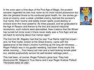
1. In the once upon a time days of the First Age of Magic, the prudent sorcerer regarded his own true name as his most valued possession but also the greatest threat to his continued good health, for--the stories go--once an enemy, even a weak unskilled enemy, learned the sorcerer's true name, then routine and widely known spells could destroy or enslave even the most powerful. As times passed, and we graduated to the Age of Reason and thence to the first and second industrial revolutions, such notions were discredited. Now it seems that the Wheel has turned full circle (even if there never really was a First Age) and we are back to worrying about true names again: The first hint Mr. Slippery had that his own True Name might be known--and, for that matter, known to the Great Enemy--came with the appearance of two black Lincolns humming up the long dirt driveway ... Roger Pollack was in his garden weeding, had been there nearly the whole morning.... Four heavy-set men and a hard-looking female piled out, started purposefully across his well-tended cabbage patch.… This had been, of course, Roger Pollack's great fear. They had discovered Mr. Slippery's True Name and it was Roger Andrew Pollack TIN/SSAN 0959-34-2861.

2. Similarity Joins for Strings and Sets William Cohen

3. Semantic Joiningwith MultiscaleStatistics William Cohen Katie Rivard, Dana Attias-Moshevitz CMU

4. WHIRL queries • “Find reviews of sci-fi comedies [movie domain] FROM review SELECT * WHERE r.text~’sci fi comedy’ (like standard ranked retrieval of “sci-fi comedy”) • ““Where is [that sci-fi comedy] playing?” FROM review as r, LISTING as s, SELECT * WHERE r.title~s.title and r.text~’sci fi comedy’ (best answers: titles are similar to each other – e.g., “Hitchhiker’s Guide to the Galaxy” and “The Hitchhiker’s Guide to the Galaxy, 2005”and the review text is similar to “sci-fi comedy”)

5. Aside: Why WHIRL’s query language was cool • Combination of cascading queries and getting top-k answers is very useful • Highly selective queries: • system can apply lots of constraints • user can pick from a small set of well-constrained potential answers • Very broad queries: • system can cherry-pick and get the easiest/most obvious answers • most of what the user sees is correct • Similar to joint inference schemes • Can handle lots of problems • classification,

15. Epilogue • A few followup query systems to WHIRL • ELIXIR, iSPARQL, … • “Joint inference” trick mostly ignored • and/or rediscovered over and over • Lots and lots of work on similarity/distance metrics and efficient similarity joins • much of which rediscovers A*-like tricks

16. Outline • Why joins are important • Why similarity joins are important • Useful similarity metrics for sets and strings • Fast methods for K-NN and similarity joins • Blocking • Indexing • Short-cut algorithms • Parallel implementation

17. Robust distance metrics for strings • Kinds of distances between s and t: • Edit-distance based (Levenshtein, Smith-Waterman, …): distance is cost of cheapest sequence of edits that transform s to t. • Term-based (TFIDF, Jaccard, DICE, …): distance based on set of words in s and t, usually weighting “important” words • Which methods work best when?

18. Edit distances • Common problem: classify a pair of strings (s,t) as “these denote the same entity [or similar entities]” • Examples: • (“Carnegie-Mellon University”, “Carnegie Mellon Univ.”) • (“Noah Smith, CMU”, “Noah A. Smith, Carnegie Mellon”) • Applications: • Co-reference in NLP • Linking entities in two databases • Removing duplicates in a database • Finding related genes • “Distant learning”: training NER from dictionaries

19. Edit distances: Levenshtein • Edit-distance metrics • Distance is shortest sequence of edit commands that transform s to t. • Simplest set of operations: • Copy character from s over to t • Delete a character in s (cost 1) • Insert a character in t (cost 1) • Substitute one character for another (cost 1) • This is “Levenshtein distance”

20. Levenshtein distance - example • distance(“William Cohen”, “WillliamCohon”) s alignment t op cost

21. Levenshtein distance - example • distance(“William Cohen”, “Willliam Cohon”) s gap alignment t op cost

22. D(i-1,j-1), if si=tj//copy D(i-1,j-1)+1, if si!=tj //substitute D(i-1,j)+1 //insert D(i,j-1)+1 //delete = min Computing Levenshtein distance - 1 D(i,j) = score of best alignment from s1..si to t1..tj

23. Computing Levenshtein distance - 2 D(i,j) = score of best alignment from s1..si to t1..tj D(i-1,j-1) + d(si,tj) //subst/copy D(i-1,j)+1 //insert D(i,j-1)+1 //delete = min (simplify by letting d(c,d)=0 if c=d, 1 else) also let D(i,0)=i(for i inserts) and D(0,j)=j

24. = D(s,t) Computing Levenshtein distance - 3 D(i-1,j-1) + d(si,tj) //subst/copy D(i-1,j)+1 //insert D(i,j-1)+1 //delete D(i,j)= min

25. Jaro-Winkler metric • Very ad hoc • Very fast • Very good on person names • Algorithm sketch • characters in s,t “match” if they are identical and appear at similar positions • characters are “transposed” if they match but aren’t in the same relative order • score is based on numbers of matching and transposed characters • there’s a special correction for matching the first few characters

26. Set-based distances • TFIDF/Cosine distance • after weighting and normalizing vectors, a dot product • Jaccard distance • Dice • …

27. Robust distance metrics for strings SecondString (Cohen, Ravikumar, Fienberg, IIWeb 2003): • Java toolkit of string-matching methods from AI, Statistics, IR and DB communities • Tools for evaluating performance on test data • Used to experimentally compare a number of metrics

28. Results: Edit-distance variants Monge-Elkan (a carefully-tuned Smith-Waterman variant) is the best on average across the benchmark datasets… 11-pt interpolated recall/precision curves averaged across 11 benchmark problems

29. Results: Edit-distance variants But Monge-Elkan is sometimes outperformed on specific datasets Precision-recall for Monge-Elkan and one other method (Levenshtein) on a specific benchmark

30. SoftTFDF: A robust distance metric • We also compared edit-distance based and term-based methods, and evaluated a new “hybrid” method: • SoftTFIDF, for token sets S and T: • Extends TFIDF by including pairs of words in S and T that “almost” match—i.e., that are highly similar according to a second distance metric (the Jaro-Winkler metric, an edit-distance like metric).

32. Comparing token-based, edit-distance, and hybrid distance metrics SFS is a vanilla IDF weight on each token (circa 1959!)

33. SoftTFIDF is a Robust Distance Metric

34. Outline • Why joins are important • Why similarity joins are important • Useful similarity metrics for sets and strings • Fast methods for K-NN and similarity joins • Blocking • Indexing • Short-cut algorithms • Parallel implementation

35. Blocking • Basic idea: • heuristically find candidate pairs that are likely to be similar • only compare candidates, not all pairs • Variant 1: • pick some features such that • pairs of similar names are likely to contain at least one such feature (recall) • the features don’t occur too often (precision) • example: not-too-frequent character n-grams • build inverted index on features and use that to generate candidate pairs

36. Blocking in MapReduce • For each string s • For each char 4-gram g in s • Output pair (g,s) • Sort and reduce the output: • For each g • For each value s associated with g • Load first K value into memory buffer • If buffer was big enough: • output (s,s’) for each distinct pair of s’s. • Else • skip this g

37. Blocking • Basic idea: • heuristically find candidate pairs that are likely to be similar • only compare candidates, not all pairs • Variant 2: • pick some numeric feature f such that similar pairs will have similar values of f • example: length of string s • sort all strings s by f(s) • Go through sorted list, and output all pairs with similar values • use a fixed-size sliding window over the sorted list

38. Key idea: • try and find all pairs x,y with similarity over a fixed threshold • use inverted indices and exploit fact that similarity function is a dot product

39. A* (best-first) search for best K paths • Find shortest path between start n0and goal ng:goal(ng) • Define f(n) = g(n) + h(n) • g(n) = MinPathLength(n0,n)| • h(n) =lower-bound of path length from n to ng • Algorithm: • OPEN= {n0} • While OPEN is not empty: • remove “best” (minimal f) node n from OPEN • if goal(n), output path n0n • and stop if you’ve output K answers • otherwise, add CHILDREN(n) to OPEN • and record their MinPathLengthparents • …note this is easy for a tree h is “admissible” and A* will always return the K lowest-cost paths

40. A* (best-first) search for good paths • Find all paths shorter than t between start n0and goal ng:goal(ng) • Define f(n) = g(n) + h(n) • g(n) = MinPathLength(n0,n)| • h(n) =lower-bound of path length from n to ng • Algorithm: • OPEN= {n0} • While OPEN is not empty: • remove “best” (minimal f) node n from OPEN • if goal(n), output path n0n • and stop if you’ve output K answers • otherwise, add CHILDREN(n) to OPEN • unless there’s no way its score will be low enough h is “admissible” and A* will always return the K lowest-cost paths

41. Build index on-the-fly • When finding matches for x consider y before x in ordering • Keep x[i] in inverted index for i • so you can find dot product dot(x,y) without using y

42. maxweighti(V) * x[i] >= best score for matching on i x[i] should be x’ here – x’ is the unindexed part of x • Build index on-the-fly • only index enough of x so that you can be sure to find it • score of things only reachable by non-indexed fields < t • total mass of what you index needs to be large enough • correction: • indexes no longer have enough info to compute dot(x,y) • ordering commonrare features is heuristic (any order is ok)

43. Order all the vectors x by maxweight(x) – now matches yto indexed parts of xwill have lower “best scores for i”

44. best score for matching the unindexed part of x update to reflect the all-ready examined part of x • Trick 1: bound y’s possible score to the unindexedpart of x, plus the already-examined part of x, and skip y’s if this is too low

45. upper bound on dot(x,y’) • Trick 2: use cheap upper-bound to see if yis worthy of having dot(x,y) computed.

46. y is too small to match x well really we will update a start counter for I • Trick 3: exploit this fact: ifdot(x,y)>t, then |y|>t/maxweight(x)

47. Large data version • Start at position 0 in the database • Build inverted indexes till memory is full • Say at position m<<n • Then switch to match-only mode • Match rest of data only to items up to position m • Then restart the process at position m instead of position 0 and repeat…..

48. Experiments • QSC (Query snippet containment) • term a in vector for b if a appears >=k times in a snippet using search b • 5M queries, top 20 results, about 2Gb • Orkut • vector is user, terms are friends • 20M nodes, 2B non-zero weights • need 8 passes over data to completely match • DBLP • 800k papers, authors + title words

49. Results

50. Results