Feature Selection, Feature Extraction
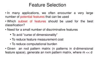
Feature Selection, Feature Extraction. Need for reduction. Classification of leukemia tumors from microarray gene expression data 1 72 patients (data points) 7130 features (expression levels of different genes) Text mining, document classification features are words


Feature Selection, Feature Extraction
E N D
Presentation Transcript
Need for reduction • Classification of leukemia tumors from microarray gene expression data1 • 72 patients (data points) • 7130 features (expression levels of different genes) • Text mining, document classification • features are words • Quantitative Structure-Activity Relationship (QSAR) • features are molecular descriptors, there exist plenty of them 1 Xing, Jordan, Karp, Feature Selection for High-Dimensional Genomic Microarray Data, 2001
QSAR • biological activity • an expression describing the beneficial or adverse effects of a drug on living matter • Structure-Activity Relationship (SAR) • hypotheses that similar molecules have similar activities • molecular descriptor • mathematical procedure transforms chemical information encoded within a symbolic representation of a molecule into a useful number
Molecular descriptor adjacency (connectivity) matrix total adj. index AV– sum all aij measure of the graph connectedness Randic connectivity indices measure of the molecular branching 2.183
QSAR • Form a mathematical/statistical relationship (model) between structural (physiochemical) properties and activity. • The mathematical expression can then be used to predict the biological response of other chemical structures. biological activity descriptor
Selection vs. Extraction • In feature selection we try to find the best subset of the input feature set. • In feature extraction we create new features based on transformation or combination of the original feature set. • Both selection and extraction lead to the dimensionality reduction. • No clear cut evidence that one of them is superior to the other on all types of task.
Why to do it? • We’re interested in features – we want to know which are relevant. If we fit a model, it should be interpretable. • facilitate data visualization and data understanding • reduce experimental costs (measurements) • We’re interested in prediction – features are not interesting in themselves, we just want to build a good predictor. • faster training • defy the curse of dimensionality
Classification of FS methods • Filter • Assess the relevance of features only by looking at the intrinsic properties of the data. • Usually, calculate the feature relevance score and remove low-scoring features. • Wrapper • Bundle the search for best model with the FS. • Generate and evaluate various subsets of features. The evaluation is obtained by training and testing a specific ML model. • Embedded • The search for an optimal subset is built into the classifier construction (e.g. decision trees).
Filter methods • Two steps (score-and-filter approach) • assess each feature individually for ist potential in discriminating among classes in the data • features falling beyong threshold are eliminated • Advantages: • easily scale to high-dimensional data • simple and fast • independent of the classification algorithm • Disadvantages: • ignore the interaction with the classifier • most techniques are univariate (each feature is considered separately)
Scores in filter methods • Distance measures • Euclidean distance • Dependence measures • Pearson correlation coefficient • χ2-test • t-test • AUC • Information measures • information gain • mutual information • complexity: O(d)
Wrappers • Search for the best feature subset in combination with a fixed classification method. • The goodness of a feature subset is determined using cross-validation (k-fold, LOOCV) • Advantages: • interaction between feature subset and model selection • take into account feature dependencies • generally more accurate • Disadvantages: • higher risk of overfitting than filter methods • very computationally intensive
Exhaustive search • Evaluate all possible subsets using exhaustive search – this leads to the optimum subset. • For a total of d variables, and subset of size p, the total number of possible subsets is • complexity: O(2d) (exponential) • Various strategies how to reduce the search space. • They are still O(2d), but much faster (at least 1000-times) • e.g. “branch and bound” e.g. d = 100, p = 10 → ≈2×10¹³
Stochastic • Genetic algorithms • Simulated Annealing
Difficulty in Searching Global Optima barrier to local search starting point descend direction local minima global minima Introduction to Simulated Annealing, Dr. Gildardo Sánchez ITESM Campus Guadalajara
Consequences of the Occasional Ascents desired effect Help escaping the local optima. adverse effect Might pass global optima after reaching it Introduction to Simulated Annealing, Dr. Gildardo Sánchez ITESM Campus Guadalajara
Simulated annealing • Slowly cool down a heated solid, so that all particles arrange in the ground energy state. • At each temperature wait until the solid reaches its thermal equilibrium. • Probability of being in a state with energy E: E … energy T … temperature kB … Boltzmann constant Z(T) … normalization factor
Cooling simulation Metropolis, 1953 Metropolis algorithm • At a fixed temperature T: • Perturb (randomly) the current state to a new state • E is the difference in energy between current and new state • If E < 0 (new state is lower), accept new state as current state • If E 0 , accept new state with probability • Eventually the systems evolves into thermal equilibrium at temperature T • When equilibrium is reached, temperature T can be lowered and the process can be repeated
Simulated annealing • Same algorithm can be used for combinatorial optimization problems: • Energy E corresponds to the objective function C • Temperature Tis parameter controlled within the algorithm
Algorithm initialize; REPEAT REPEAT perturb ( config.i config.j, Cij); IF Cij < 0 THEN accept ELSE IF exp(-Cij/T) > random[0,1) THEN accept; IF accept THEN update(config.j); UNTIL equilibrium is approached sufficient closely; T := next_lower(T); UNTIL system is frozen or stop criterion is reached
Parameters • Choose the start value of T so that in the beginning nearly all perturbations are accepted (exploration), but not too big to avoid long run times • At each temperature, search is allowed to proceed for a certain number of steps, L(k). • The function next_lower (T(k)) is generally a simple function to decrease T, e.g. a fixed part (80%) of current T.
At the end T is so small that only a very small number of the perturbations is accepted (exploitation). • The choice of parameters {T(k), L(k)} is called the cooling schedule. • If possible, always try to remember explicitly the best solution found so far; the algorithm itself can leave its best solution and not find it again.
Deterministic • Sequential Forward Selection (SFS) • Sequential Backward Selection (SBS) • “ Plus qtake away r ” Selection • Sequential Forward Floating Search (SFFS) • Sequential Backward Floating Search (SBFS)
Sequential Forward Selection • SFS • At the beginning select the best feature using a scalar criterion function. • Add one feature at a time which along with already selected features maximizes the criterion function. • A greedy algorithm, cannot retract (also called nesting effect). • Complexity is O(d)
Sequential Backward Selection • SBS • At the beginning select all d features. • Delete one feature at a time and select the subset which maximize the criterion function. • Also a greedy algorithm, cannot retract. • Complexity is O(d).
“Plus q take away r” Selection • At first add q features by forward selection, then discard r features by backward selection • Need to decide optimal q and r • No subset nesting problems Like SFS and SBS
Sequential Forward Floating Search • SFFS • It is a generalized “plus q take away r” algorithm • The value of q and r are determined automatically • Close to optimal solution • Affordable computational cost • Also in backward disguise
Embedded FS • The feature selection process is done inside the ML algorithm. • Decision trees • In final tree, only a subset of features are used • Regularization • It effectively “shuts down” unnecessary features. • Pruning in NN.
FS – indetify and select the “best” features with respect to the target task. • Selected features retain their original physical interpretation. • FE – create new features as a transformation (combination) of original features. Usually followed by FS. • May provide better discriminatory ability than the best subset. • Do not retain the original physical interpretation, may not have clear meaning.
x2 x1
x2 Make data to have zero mean (i.e. move data into [0, 0] point). centering x1
x2 This is a line given by equation w0 + w1x1 + w2x2 This is another line w’0 + w’1x1 + w’2x2 x1
The variability in data is highest along this line. It is called 1st principal component. x2 And this is 2nd principal component. x1
x2 Principal components (PC’s) are linear combinations of original coordinates. The coefficients of linear combination (w0, w1, …) are called loadings. In the transformed coordinate system, individual data points have different coordinates, these are called scores. w0 + w1x1 + w2x2 w’0 + w’1x1 + w’2x2 x1
PCA - orthogonal linear transformation that changes the data into a new coordinate system such that the variance is put in order from the greatest to the least. • Solve the problem = find new orthogonal coordinate system = find loadings • PC’s (vectors) and their corresponding variances (scalars) are found by eigenvalue decompositions of the covariance matrix C = XXT of the xi variables. • Eigenvector corresponding to the largest eigenvalue is 1st PC. • The 2nd eigenvector (the 2nd largest eigenvalue) is orthogonal to the 1st one. … • Eigenvalue decomposition is computed using standard algorithms: eigen decomposition of covariance matrix (e.g. QR algorithm), SVD of mean centered data matrix.
Interpretation of PCA • New variables (PCs) have a variance equal to their corresponding eigenvalue Var(Yi)=i for all I = 1…p • Smalli small variance data changes little in the direction of componentYi • The relative variance explained by each PC is given by li / li
How many components? • Enough PCs to have a cumulative variance explained by the PCs that is >50-70% • Kaiser criterion: keep PCs with eigenvalues >1 • Scree plot: represents the ability of PCs to explain de variation in data