Feature Selection
Feature selection plays a critical role in data analysis, particularly in reducing the dimensionality of datasets. Not all features contribute positively; some may introduce noise and reduce the model's accuracy. Methods such as stepwise approaches help identify the most relevant features that are closely associated with outcomes, especially in genetics and cancer research. Principal Component Analysis (PCA) simplifies datasets by transforming groups of correlated variables into orthogonal components, capturing the majority of the variance. This allows researchers to focus on key driving forces in their data.

Feature Selection
E N D
Presentation Transcript
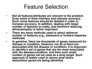
Feature Selection • Not all features/attributes are relevant to the problem. Even some of them interfere and reduces accuracy. Such noisy features should be deleted in order to increase accuracy. In addition, dealing with larger number of features is costly, and therefore reducing dimensionality is rather important. • There are many methods used to select optimum number of features (e.g., backward or forward stepwise methods) • In genetics, there are thousands of genes measured for disease or condition. However, not all of them are associated with the disease or condition. It is important to identity a set of genes that are the most associated with the disease/condition, and then such small number of genes can be used as a drug target. Such approach is widely used in cancer area where associative genes are being identified.
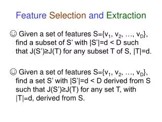
Feature Selection Optimal solution is to try all possible combinations of the features (=2m-1)
Feature Selection Methods IEEE PAMI, 2000, 22(1):4-37
Some other methods for feature selection available in MATLAB
Feature Extraction and Projection Methods IEEE PAMI, 2000, 22(1):4-37
Principalcomponentsanalysis In data sets with many variables, groups of variables often move together. One reason for this is that more than one variable might be measuring the same driving principle governing the behavior of the system. In many systems there are only a few such driving forces. But an abundance of instrumentation enables you to measure dozens of system variables. When this happens, you can take advantage of this redundancy of information. You can simplify the problem by replacing a group of variables with a single new variable. Principal components analysis is a quantitatively rigorous method for achieving this simplification. The method generates a new set of variables, called principal components. Each principal component is a linear combination of the original variables. All the principal components are orthogonal to each other, so there is no redundant information. The principal components as a whole form an orthogonal basis for the space of the data.
There are an infinite number of ways to construct an orthogonal basis for several columns of data. • The first principal component is a single axis in space. When you project each observation on that axis, the resulting values form a new variable. And the variance of this variable is the maximum among all possible choices of the first axis. • The second principal component is another axis in space, perpendicular to the first. Projecting the observations on this axis generates another new variable. The variance of this variable is the maximum among all possible choices of this second axis. • The full set of principal components is as large as the original set of variables. But it is commonplace for the sum of the variances of the first few principal components to exceed 80% of the total variance of the original data. By examining plots of these few new variables, researchers often develop a deeper understanding of the driving forces that generated the original data.