Understanding Classification: Naïve Bayes and Nearest-Neighbor Classifiers Explained
170 likes | 285 Vues
This lecture outlines the foundational concepts of classification in machine learning, focusing on the Naïve Bayes classifier and the k-nearest neighbors (k-NN) classifier. It contrasts eager and lazy learners, explaining how eager learners build models immediately upon receiving data, while lazy learners defer this until necessary. The session delves into distance measures like Euclidean and Jaccard distances for k-NN and covers Bayes Theorem for computing conditional probabilities. It highlights characteristics and advantages of Naïve Bayes, including its robustness to noise and its capacity to handle missing data.

Understanding Classification: Naïve Bayes and Nearest-Neighbor Classifiers Explained
E N D
Presentation Transcript
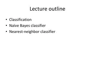
Lecture outline • Classification • Naïve Bayesclassifier • Nearest-neighbor classifier
Eager vs Lazy learners • Eager learners: learn the model as soon as the training data becomes available • Lazy learners: delay model-building until testing data needs to be classified • Rote classifier: memorizes the entire training data
k-nearest neighbor classifiers k-nearest neighbors of a record x are data points that have the k smallest distance to x
k-nearest neighbor classification • Given a data record x find its k closest points • Closeness: Euclidean, Hamming, Jaccard distance • Determine the class of x based on the classes in the neighbor list • Majority vote • Weigh the vote according to distance • e.g., weight factor, w = 1/d2 • Probabilistic voting
Characteristics of nearest-neighbor classifiers • Instance of instance-based learning • No model building (lazy learners) • Lazy learners: computational time in classification • Eager learners: computational time in model building • Decision trees try to find global models, k-NN take into account local information • K-NN classifiers depend a lot on the choice of proximity measure
Bayes Theorem • X, Y random variables • Joint probability: Pr(X=x,Y=y) • Conditional probability: Pr(Y=y | X=x) • Relationship between joint and conditional probability distributions • Bayes Theorem:
Bayes Theorem for Classification • X: attribute set • Y: class variable • Y depends on X in a non-determininstic way • We can capture this dependence using Pr(Y|X) : Posterior probability vs Pr(Y): Prior probability
Building the Classifier • Training phase: • Learning the posterior probabilities Pr(Y|X) for every combination of X and Y based on training data • Test phase: • For test record X’, compute the class Y’ that maximizes the posterior probability Pr(Y’|X’)
BayesClassification: Example X’=(Home Owner=No, Marital Status=Married, AnnualIncome=120K) Compute: Pr(Yes|X’), Pr(No|X’) pick No or Yes with max Prob. How can we compute these probabilities??
Computing posterior probabilities • Bayes Theorem • P(X) is constant and can be ignored • P(Y): estimated from training data; compute the fraction of training records in each class • P(X|Y)?
Naïve Bayes Classifier • Attribute set X = {X1,…,Xd} consists of d attributes • Conditional independence: • X conditionally independent of Y, given X: Pr(X|Y,Z) = Pr(X|Z) • Pr(X,Y|Z) = Pr(X|Z)xPr(Y|Z)
Naïve Bayes Classifier • Attribute set X = {X1,…,Xd} consists of d attributes
Conditional probabilities for categorical attributes • Categorical attribute Xi • Pr(Xi = xi|Y=y): fraction of training instances in class y that take value xion the i-th attribute • Pr(homeOwner = yes|No) = 3/7 • Pr(MaritalStatus = Single| Yes) = 2/3
Estimating conditional probabilities for continuous attributes? • Discretization? • How can we discretize?
Naïve Bayes Classifier: Example • X’ = (HomeOwner = No, MaritalStatus = Married, Income=120K) • Need to compute Pr(Y|X’) or Pr(Y)xPr(X’|Y) • But Pr(X’|Y) is • Y = No: • Pr(HO=No|No)xPr(MS=Married|No)xPr(Inc=120K|No) = 4/7x4/7x0.0072 = 0.0024 • Y=Yes: • Pr(HO=No|Yes)xPr(MS=Married|Yes)xPr(Inc=120K|Yes) = 1x0x1.2x10-9 = 0
Naïve Bayes Classifier: Example • X’ = (HomeOwner = No, MaritalStatus = Married, Income=120K) • Need to compute Pr(Y|X’) or Pr(Y)xPr(X’|Y) • But Pr(X’|Y = Yes) is 0? • Correction process: nc: number of training examples from class yj that take value xi n: total number of instances from class yj m: equivalent sample size (balance between prior and posterior) p: user-specified parameter (prior probability)
Characteristics of Naïve Bayes Classifier • Robust to isolated noise points • noise points are averaged out • Handles missing values • Ignoring missing-value examples • Robust to irrelevant attributes • If Xi is irrelevant, P(Xi|Y) becomes almost uniform • Correlated attributes degrade the performance of NB classifier

