A Tutorial on Helical Structures
A Tutorial on Helical Structures. David DeRosier W.M. Keck Institute for Cellular Visualization Brandeis University. An example of a helical structure. There are also helical biological structures:. Rod-shaped viruses. Actin filaments. Microtubules. Intermediate filaments.


A Tutorial on Helical Structures
E N D
Presentation Transcript
A Tutorial on Helical Structures David DeRosier W.M. Keck Institute for Cellular Visualization Brandeis University
There are also helical biological structures: Rod-shaped viruses Actin filaments Microtubules Intermediate filaments Myosin filaments Bacterial pili
How can we study helical structures? X-ray fiber diffraction? 1. It is difficult to get good preparations and the analysis is also difficult. 2. It can potentially provide atomic resolution (~3A) but tobacco mosaic virus is the only structure solved to this resolution using the general method of isomorphous replacement.
Electron microscopy is the method of choice. It is routine to achieve a resolution of 20 A. 1. At this resolution one can visualize subunits and even domains. 2. This resolution is sufficient to permit quite accurate docking of atomic models for the subunits into maps. Several structures have been solved 8-10 A allowing one to see alpha helices. One structure, the acetylcholine receptor has been solved to 4.6 A, where one might be able to trace the backbone.
We can predict that electron microscopy will continue to be the method of choice for helical particles. We predict that the methodology will continue to be improved so that near atomic resolution will be possible for at least some structures. But we must be cautious about making predictions:
“It’s hard to make predictions, especially about the future.” Yogi Berra
Today’s example is a helical component of the bacterial flagellum.
Negatively stained image showing the helical parts of a bacterial flagellum. Filament Hook Rod Electron Micrograph (DePamphilis & Adler, 1960s).
How do we generate a three dimensional map of a structure with helical symmetry? Whether a structure has helical symmetry of not, we combine images corresponding to different views of the structure. But helical structures are special. Often only one view is needed! How can that be?
A helical particle consists of a set of identical subunits arranged on a helical lattice. The subunits are oriented at equally spaced angles. Thus a single image of a helical structure can have all views of the subunit needed to generate a three dimensional map.
But to produce a 3D map, we have to know the position and angular orientation of every subunit; i.e., we need to go into the helical symmetry rules! And you need to know where your going when it comes to determining helical symmetry.
You’ve got to be very careful if you don’t know where you’re going because you might not get there. - Yogi Berra
Most of the computer programs needed to convert images into a 3D map are automated or semi-automated, but … the key step needed to initiate the use of these computer programs is a determination of the helical symmetry. We will begin with this.
It looks simple to determine the symmetry of our model just from looking at its image, but how about a real structure?
The hook of the bacterial flagellum, a helical assembly of protein subunits. 100 nm
What do we do to determine the helical symmetry if we can’t determine it by inspection of the image? We begin by calculating the Fourier transform of a digitized image.
This is the Fourier transform of our model helix. Only the top half is shown because the bottom half is identical (due to Friedel’s law). The transform of a helical structure consists or strong reflections that lie on a series of regularly spaced lines called layer lines.
This is the (whole) Fourier transform of the hook. 4 3 2 1 e There are 4 layer lines plus the equator. There are in fact many more layer lines but they are hidden by noise
To determine the helical symmetry: 1. We determine the positions of all the layer lines.
The axial positions of the layer lines can be selected approximately by eye, but these positions obey strict rules. Layer lines obey the same positional rules as reflections from a 2D crystal as we shall see.
The Fourier transform of a helix looks like the Fourier transform of a 2D lattice but everything appears doubled!
meridian equator Each layer line haspairs of spotsplaced symmetrically about the meridian. The innermost spots on each layer line form two approximate lattices one arising from the the nearside of the helix (the side closer to the viewer) and the other from the far side.
2D lattice Fourier transform of this lattice.
Isn’t it hard to figure out which reflections belong to which lattice? Not necessarily. Often there are only two choices.
1. Choose two layer lines near the origin. 2. Pick the innermost spot on one side of one of them. 3. Pick one of two innermost spots on the other. 4. Draw the lattice defined by these two spots. In this case, we chose incorrectly, and the wrong choice results in a lattice that fails to go through all the (first) maxima of the layer lines.
Instead of choosing the right side spot, we try the left-side spot
Okay, you say, but let’s see if this theoretical strategy works in practice on the hook. In theory, there is no difference between theory and practice. In practice, there is.
The wrong choice results in a lattice that misses strong layer lines. The other choice does!
The correct choice does identify the layer lines giving the two (near- and far-side) lattices.
We made too many wrong mistakes. Luckily, there are only two choices. So usually you can only make one wrong mistake.
To determine the helical symmetry. 1. We determine the positions of all the layer lines. 2. We next determine the order of each layer line.
Each layer line arises from a family of helical lattice lines. For example, the family highlighted in yellow gives rise to the highlighted layer line. The order of the layer line is equal to the number of continuous lines in the family; in this case there is one. n=1
This number is also equal to the number of times the family crosses an equatorial plane or line. This can be seen most easily in the unrolled helical net.
Here is another helical family, which crosses 11 times. Thus its order is n=11.
Here are the lattice lines drawn onto our model. They are very steep lines. They give rise to the layer line closest to the equator. The order of this layer line is eleven. n=11
How does one determine the order, n, for each layer line if one knows nothing to start with? One can get an approximate order of each layer line and one can determine whether the order is odd or even. These can be enough to determine the order exactly.
r d The number of lattice lines (which equals the order, n) is equal to the circumference of the helix divided by the distance between lattice lines: n=2pr/d We can determine the value of r by measuring the width of the particle. But how can we measure d?
If we measure R, the distance from the meridian to the first major reflection, we have essentially determined d; that is d ~ 1/R. A more exact formula is: 2 p r R ~ n + 2 for n > 4 d R
Because of errors, it is best to estimate the orders of layer lines whose maxima are closest to the meridian; these have the smallest n. 2R4 2R3 4 3 2 1 0 2r For layer lines 3 and 4, we measure R. From the image of the hook, we measure r.
Here is what was actually determined for the hook: Layer line #3, n=2 p r R –2 = 6.4 and thus n = 6 or 7. Layer line #4, n=2 p r R - 2= 4.6 and thus n = 4 or 5. How can one pick between the possibilities?
Dq4 Dq3 4 3 2 1 0 We can determine whether n is odd or even and thus we can distinguish between 4 vs 5 or 6 vs 7. To do so we use the phases determined in the Fourier transforms of the image. We calculate the phase differences between pairs of reflections symmetric about the meridian. Thus we measure Dq3= q3,L- q3R for layer line #3 and the same for layer line #4. If Dq ~ 180o, n is odd; if Dq ~ 0o , n is even!
Here is what was found: For layer line #3, n = 6 or 7, but Dq 3 ~ 11o and hence n is even and n=6. For layer line #4, n = 4 or 5, but Dq 4~ 163o and hence n is odd and n=5.
With our measurements of layer line heights and orders, we can draw lattice in which we plot n, layer line order, vs. l, layer line height for the layer lines. These points form a perfect lattice and hence predict the positions and orders of all possible the layer lines arising from this helical symmetry.
Here the “known” 4 layer lines are indicated as filled black circles and a few of the predicted ones are shown as open circles. l n
The height of each layer line gives us a measure of the pitch, p, of the corresponding lattice lines and from that we can construct the helical lattice. l 1/p6 1/p11 n
Notice that some of our points in the n,l plot have negative values of n (e.g., n=-11). The convention is that n>0 refers to right-handed helical families and n<0 to left-handed families. For our plot, we have chosen two pairs of helical families n= -11, l=1/148Å and n= +6, l=1/53Å, but we don’t yet know the absolute hand of the structure. So it could also be that n= +11, l=1/148Å and n= -6, l=1/53Å.