Pyro-convective cloud from aircraft ~ 10km (N57, W125) June 27, 2004

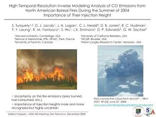
1. High Temporal Resolution Inverse Modeling Analysis of CO Emissions from North American Boreal Fires During the Summer of 2004 Importance of Their Injection Height S. Turquety1,2, D. J. Jacob1, J. A. Logan1, C. L. Heald4, D. B. Jones3, R. C. Hudman1, F. Y. Leung1, R. M. Yantosca1, S. Wu1, L.K. Emmons5, D. P. Edwards5, G. W. Sachse6 4University of California Berkeley, USA 5NCAR, Boulder, USA 6NASA Langley Research Center, Hampton, USA 1Harvard University, Cambridge, USA 2Service d’Aéronomie, IPSL, UPMC, Paris, France 3University of Toronto, Canada • Uncertainty on the fire emissions (area burned, fuel consumed, etc.) • Importance of injection heights more and more recognized but highly uncertain Pyro-convective cloud from aircraft ~ 10km (N57, W125)June 27, 2004 www.cpi.com/remsensing/midatm/smoke.html Solène Turquety – AGU fall meeting, San Francisco, December 2006

2. 19 Tg 11 Tg Daily inventory of boreal fire emissions for North America in 2004 (Turquety et al., submitted, JGR) Summer of 2004: Largest fire year on record in terms of area burned in Alaska and western Canada; Pfister et al., GRL, 2005: Inverse modeling a posteriori estimate 30 ± 5 Tg CO emitted based on MOPITT CO ~ twice their a priori estimate • We constructed a daily area burned: • Temporal variability: daily reports from the U.S. National Interagency Fire Center • Location of the fires: MODIS hotspot detection • Fuel consumption and emission factors including the contribution from peat burning Solène Turquety – AGU fall meeting, San Francisco, December 2006

3. MOPITT Model with peat Model without peat Evaluation using the MOPITT CO observations (Turquety et al., submitted, JGR) GEOS-Chem: no peat burning GEOS-Chem: with peat burning • Highlights the importance of peat burning • Strong uncertainty remain: • Areas burned/Timing of fires? • Fuel consumption? • Impact of injection heights? Solène Turquety – AGU fall meeting, San Francisco, December 2006

4. Variability CO emissions and max TOMS AI Alaska-Yukon [165-125W] Importance of high altitude injection in 2004 • Several studies have shown that pyro-convective events occurred – and could explain some long-range transport events : e.g. • Damoah et al., 2006 : event end of June • DeGouw et al., 2006 : event in mid-July • Peaks in TOMS AI suggest pyro-convection events: end of June, beginning of July, mid-July and mid-August • Average vertical distribution of boreal fires emissions in the CTM (F-Y Leung): • 40% boundary layer • 30% FT ~ [600–400hPa] • 30% UT ~ [400–200hPa] Solène Turquety – AGU fall meeting, San Francisco, December 2006

5. MOPITT CO – summer 2004 GEOS-Chem CO * MOPITT AK + Gain matrix (MOPITT – MODEL) Inverse modeling of boreal fire emissions Forward model: Observations: Inversion a posteriori estimates a priori sources xa Maximum a posteriori solution (Rodgers, 2000) With S∑ : observation and model error Sa : a priori error K : Jacobians (∂y/ ∂x) Solène Turquety – AGU fall meeting, San Francisco, December 2006

6. Kalman Filter Kalman Smoother Analysis update Analysis Analysis Time dependant inversion using a Kalman smoother Initial conditions = MOPITT CO assimilation (D. Jones, U. Toronto) Kalman smoother: observations from ‘future’ also used to update emissions Solène Turquety – AGU fall meeting, San Francisco, December 2006

7. GEOS-Chem CO * MOPITT AK Time dependant inversion using a Kalman smoother Observations influenced by emissions for current day but also past emissions! Separate contribution from different time steps in the model Jacobian K now time dependant: with t0 t Fixed update Each emission time step update P times, last estimate = best estimate Emissions during 3 days (1 timestep); P = 5 timesteps updated (5 x 3 = 15 days) Solène Turquety – AGU fall meeting, San Francisco, December 2006

8. Model pulse simulations including vertical distribution of the emissions GEOS-Chem model simulation to be compared to the MOPITT observations: • State vector including vertical distribution: • 3 biomass burning regions x 3 vertical regions:BL, MT, UT • North American FF/BF, Asia, Rest of the world + chemical production Decaying background : initial conditions = assimilated MOPITT CO (University of Toronto) Emissions during 3 days (1 timestep); P = 5 timesteps updated (5 x 3 = 15 days) Solène Turquety – AGU fall meeting, San Francisco, December 2006

9. Forward model K x + bckgd Observations y BB AK-YK – Middle trop. BB AK-YK – Upper trop. BB AK-YK – Boundary layer t (3 days timestep) Contribution at t from emissions at t t-1 Contribution at t from emissions at t-1 t-2 Contribution at t from emissions at t-2 Solène Turquety – AGU fall meeting, San Francisco, December 2006

10. Total CO Initial a priori uncertainty on the emissions Sa • 50% on biomass burning emissions in our region of interest • 30% on emissions for the rest of the world • 20% uncertainty on chemical production • 1st adjustment of the emissions at a given timestep => errors uncorrelated • 2nd adjustment of a given time step: Sa(t,t) = Sx(t,t-1) => introduce correlations A priori uncertainty on the observations and model Se • Determined using the method described by Heald et al., JGR, 2004 • uncertainty = observation – model • Assume correlation length scale = 147 km Maximum error over the fire region, reflecting the large uncertainties ~ 30 – 50% ~ 5 – 20 % elsewhere Solène Turquety – AGU fall meeting, San Francisco, December 2006

11. Still update… Pyroconvective event end of June Inversion of the emissions in 3 vertical regions: boundary layer (BL), middle troposphere (MT) and upper troposphere (UT) (preliminary results) A priori “vertdis”: 40% BL, 30% MT, 30%UT Sensitivity of the inversion to injection height, information seems to be available for the inversion of this parameter in parallel Solène Turquety – AGU fall meeting, San Francisco, December 2006

12. Variability CO emissions and max TOMS AI Alaska-Yukon [165-125W] Inversion of the emissions in 3 vertical regions: boundary layer (BL), middle troposphere (MT) and upper troposphere (UT) (preliminary results) A priori “vertdis”: 40% BL, 30% MT, 30%UT Sensitivity of the inversion to injection height, information seems to be available for the inversion of this parameter in parallel Solène Turquety – AGU fall meeting, San Francisco, December 2006

13. Variability CO emissions and max TOMS AI Central Canada From Alaska Inversion of the emissions in 3 vertical regions: boundary layer (BL), middle troposphere (MT) and upper troposphere (UT) (preliminary results) Large event in the beginning of August Solène Turquety – AGU fall meeting, San Francisco, December 2006

14. Conclusions and future directions • Bottom-up emissions inventory estimate of 30 Tg CO, incl. 11 Tg CO from peat burning [Turquety et al., subm., 2006] • Including peat burning allows better agreement with first top-down estimates of 30 ± 5 Tg by Pfister et al. [2005] • Injection height is important for specific events – less important on CO averaged over the summer • Injection heights have an impact on high temporal resolution top-down emissions inversions from MOPITT • Limited information on the vertical distribution in MOPITT • Information in the MOPITT transport pathways on injection height can be used to constrain this parameter • Data could be used to specify injection height together with inventories: • TOMS AI • POAM stratospheric aerosols (Fromm et al.) • MISR : see poster Fok-Yan Leung A51C-0099 • Calipso lidar in space? • Solar occultation measurements from ACE? • Efforts currently undertaken to include a physical parameterization of injection heights in models • One focus of the POLARCAT international campaign to be held in 2008 Solène Turquety – AGU fall meeting, San Francisco, December 2006

15. MODIS fire detection 20-26 July, 2006 Detection of vertical distribution over source regions and downwind with CALIPSO Courtesy J. Pelon, Service d’Aéronomie Solène Turquety – AGU fall meeting, San Francisco, December 2006

16. Solar occultation measurements from the ACE/SCISAT-1 instrument: CO (+) Large variety of species measured O3, H2O, H2O2, CO, CH4, C2H6, C2H2, HCN, CH3Cl, SF6, OCS, HNO3, PAN,… (+) Very good vertical resolution (+) Orbit scheduled sample boreal regions in July (-) Lack coverage (-) No data at altitudes < ~6km C2H6 HCN Solène Turquety – AGU fall meeting, San Francisco, December 2006