Download
1 / 82
820 likes | 941 Vues
Explore the historical, theoretical, and pragmatic perspectives on resolution needed to simulate convection in numerical weather prediction models, touching on the 1 km grid spacing standard and justifications for high-resolution modeling.

E N D
Representation of Convective Processes in NWP Models (part II) George H. Bryan NCAR/MMM Presentation at ASP Colloquium, “The Challenge of Convective Forecasting” 13 July 2006
Outline • Part I: What is a numerical model? • Part II: What resolution is needed to simulate convection in numerical models?
Part II: What resolution is needed to simulate convection in numerical models? • An interesting question. • What do our commandments say?
Commandments (continued) • Thou shalt use 1 km grid spacing to simulate convection explicitly • ….
Commandments (continued) • Thou shalt use 1 km grid spacing to simulate explicitly convection • Honor thy elders • …. “There’s no need for grid spacing smaller than 2 km.”
Perspectives on resolution • Historical Perspective • Theoretical Perspective • Pragmatic Perspective
The “1 km standard” • Often quoted in journal articles, textbooks, at conferences, etc. • Clearly, there is some veracity to this “rule of thumb” • otherwise, it wouldn’t be so common • But, where did it come from?
The first cloud models • Steiner (1973) • Perhaps first 3D simulation of convection • = 200 m • Cumulus congestus • Schlesinger (1975) • Perhaps first 3D simulation of deep convection • = 3.2 km • “a rather coarse mesh was used” • Schlesinger (1978) • = 1.8 km
The first cloud models (cont.) • Klemp and Wilhelmson (1978) • A groundbreaking paper • The KW Model is the grand-daddy of the ARW Model • = 1 km • “… this resolution is admittedly rather coarse” • Tripoli and Cotton (1980) • = 750 m • Weisman and Klemp (1982) • = 2 km • “Finer resolution would be preferable …”
Commandments (continued) • Thou shalt read the Old Testament • ….
The first cloud models (cont.) • Klemp and Wilhelmson (1978) • A groundbreaking paper • The KW Model is the grand-daddy of the ARW Model • = 1 km • “… this resolution is admittedly rather coarse” • Tripoli and Cotton (1980) • = 750 m • Weisman and Klemp (1982) • = 2 km • “Finer resolution would be preferable …”
Summary of literature review • of O(1 km) was there from the beginning • Many recognized/suggested that this was too coarse • In the decades that followed (80s and 90s), increasing computing power was utilized mainly for larger domains and longer integration times
Justification for 1 km • Not a great deal of justification out there, other than: • The Sixth Commandment • “scientist A used this resolution; thus, I can, too.” • “It’s all I could afford.” • However …
Justification for 1 km • Weisman et al. (1997) performed a large number of simulations, using from 12 km to 1 km • “… 4 km grid spacing may be sufficient to reproduce … midlatitude type convective systems” • They identified (correctly) that non-hydrostatic processes cannot be resolved unless 1 km
higher resolution higher resolution Weisman, Skamarock, and Klemp, 1997: The Resolution Dependence of Explicitly Modeled Convective Systems (MWR, pg 527) ~4 km is sufficient to simulate mesoscale convective systems System-averaged rainwater mixing ratio (qr) weak shear strong shear “Clearly, the 1-km solution has not converged.” “…grid resolutions of 500 m or less may be needed to properly resolve the cellular-scale features …”
Looking beyond 1 km • Only since the middle 90s have people looked below 1 km systematically • It’s expensive! • Need grids of O(1000 x 1000) • Small time steps • Droegemeier et al. (1994, 1996, 1997) • Found differences in simulations of supercells with 100 m • Turbulent details began to emerge
Supercell simulations: rainwater mixing ratio at z = 4 km, t = 1 h from: Droegemeier et al. (1994)
Other recent studies • Petch and Grey (2001) • Petch et al. (2002) • Adlerman and Droegemeier (2002) • Bryan et al. (2003) • All found that results were not converged with = 1 km • i.e., results are dependent on grid spacing • But why? • And what are consequences of coarse resolution?
Δx = Δz = 125 m: θe, across-line cross sections with RKW “optimal” shear Δ x = 1000 m, Δz = 500 m:
Δx = Δz = 125 m: θe, along-line cross sections with RKW “optimal” shear Δ x = 1000 m, Δz = 500 m:
along-line cross sections of θe: x=211 km, x=208 km, x=205 km
125 m: Rainwater mixing ratio with “strong” shear 1000 m:
125 m: θe, with “strong” shear 1000 m:
Perspectives on resolution • Historical Perspective • Theoretical Perspective • Pragmatic Perspective
How big are convective clouds, anyway? • Clouds are surprisingly small • Median updraft diameters are ~2-4 km • Updrafts of ~10 km are rare, and are usually found in supercells
Results of a thorough literature review from: Bryan et al. (2006)
Some of my conclusions: • Clouds are of O(1 km) • Grid spacing of O(1 km) should marginally resolve convective updrafts • I think the earliest cloud modelers knew this
The difference between resolution and grid spacing • Grid spacing () is clear • The distance between grid cells • Resolution is nebulous • Recall that numerical techniques cannot properly handle features less than ~6
Analytic solution to the advection equation • “E” = exact • “2” = 2nd order centered • “4” = 4th-order centered from: Durran (1999)
Analytic solution to the artificial diffusion terms • “2” = 2 • “4” = 4 • “6” = 6 from: Durran (1999)
Effective Resolution • This is a relatively new concept (to some) • The effective resolution of a numerical model is the minimum scale that is not affected by artificial aspects of the modeling system • In the ARW Model, this is ~6-8
Kinetic energy spectra from ARW simulations from: Skamarock (2004)
Synthesis • O(1 km) grid spacing is needed to resolve nonhydrostatic processes • Deep convective clouds are of O(1 km), and some supercells are of O(10 km) • The ARW Model needs ~6-8 to “resolve” a feature 1 km grid spacing is looking marginal
Scales in turbulent flows • L is the scale of the large eddies • e.g., a Cu cloud • is the scale of the dissipative eddies • e.g., the cauliflower-like “puffiness”
Turbulence • Small-scale turbulence cannot be resolved in numerical models • Theory is clear (Kolmogorov 1940) • To resolve all scales in clouds requires ~0.1 mm grid spacing (Corrsin 1961) • So, what should we do … ?
The filtered Navier-Stokes equations Start with: Apply a filter, rearrange terms All sub-filter-scale flow is contained in the term (the subgrid turbulent flux) from Bryan et al. (2003)
Modeling subgrid turbulence • We have a fairly good idea of how to parameterize for many flows • HOWEVER … a few rules apply
Scales in turbulent flows • L is the scale of the large eddies • e.g., a Cu cloud • is the scale of the dissipative eddies • e.g., the cauliflower-like “puffiness”
1/η 1/L Turbulence Kinetic Energy Spectrum E(κ) κ
? r s LES MM r s r s DNS r 1/Δ 1/Δ 1/Δ 1/Δ The Four Regimes of Numerical Modeling (Wyngaard, 2004) E(κ) κ
“Crude representation of average energy degradation path” (A Roadmap!) Turbulent kinetic energy (small eddies) Turbulent kinetic energy (large eddies) Mean flow kinetic energy Internal energy of fluid (heat) Corrsin (1960)
Roadmap for LES Turbulent kinetic energy (large eddies) Mean flow kinetic energy
Roadmap for LES Turbulent kinetic energy (large eddies) Mean flow kinetic energy Transfer of kinetic energy to unresolved scales
LES subgrid model • Works well if grid spacing () is 10-100 times smaller than the large eddies (L) • Recall: L~2-4 km • Suggests that needs to be ~20-200 m • If we want to use LES models … and we do … then of O(100 m) might be necessary
Early cloud modelers knew this • Klemp and Wilhelmson (1978): • “. . . closure techniques for the subgrid equations are based on the existence of a grid scale within the inertial subrange and with present resolution [Δx = 1 km] this requirement is not satisfied.”
A problem: we want to do this …. Turbulent kinetic energy (large eddies) Mean flow kinetic energy Transfer of kinetic energy to unresolved scales