Quantum random walks and quantum algorithms
Quantum random walks and quantum algorithms. Andris Ambainis University of Latvia. Part 1. Quantum walks as a mathematical object. Random walk on line. . . Start at location 0. At each step, move left with probability ½, right with probability ½. -2. -1. 0. 1. 2.

Quantum random walks and quantum algorithms
E N D
Presentation Transcript
Quantum random walks and quantum algorithms Andris Ambainis University of Latvia
Part 1 Quantum walks as a mathematical object
Random walk on line ... ... • Start at location 0. • At each step, move left with probability ½, right with probability ½. -2 -1 0 1 2 Continuous time version: move left/right at certain rate.
Cont. time quantum walk Adjacency matrix: • Random walk: • Quantum walk:
Random walk on line ... ... • State (x, d), x –location, d-direction. • At each step, • Let d=left with prob. ½, d=right w. prob. ½. • (x, left) => (x-1, left); • (x, right) => (x+1, right). -2 -1 0 1 2
Quantum walk on line ... ... -2 -1 0 1 2 • States |x, d, x –location, d-direction. “Coin flip”: Shift:
Classical vs. quantum Run for t steps, measure the final location. Distance: (t) Distance: (t)
Semi-infinite walk ... • Start at 0. • At each step, move left with probability ½, right with probability ½. • Stop, if we are at –1. • Quantum version: project out the components at |-1, left and |-1, right. 0 1 2
Semi-infinite walk [A, Bach, et al., 01] ... • What is the probability of stopping? • Classically, 1. • Quantumly, 2/. • With some probability, quantum walk “never reaches” –1. 0 1 2
Finite walk [Bach, Coppersmith, et al., 2003] ... • Start at 0. • Stop at –1 or n+1. • Classically, probability to stop at –1 is n/(n+1). • Quantumly, it tends to 1/2, for large n. n 0 1 2 Surprising, for two reasons
Probabilities to stop at -1 “Semi-infinite” is not limit of “large n” Having a faraway border increases the chance of returning to -1 1/2 > 2/
Explanation time A second boundary reflects part of the state location
H – adjacency matrix of a graph. Quantum walk on general graphs
Edges: |u, v. • “Coin flip”: • “Shift”: Discrete quantum walk
Part 2 Applications of quantum walks
Quantum search on grids [Benioff, 2000] • N* N grid. • Each location stores a value. • Find a location storing a certain value.
Grover’s search ... 0 1 0 0 • Find i for which xi=1. • Questions: ask i, get xi. • Classically, N questions. • Quantum, O(N) questions [Grover, 1996]. x1 x2 x3 xN
Quantum search on grids [Benioff, 2000] • Distance between opposite corners = 2N. • Grover’s algorithm takes steps. No quantum speedup.
Quantum search on grids • [A, Kempe, Rivosh, 2004] O(N logN) time quantum algorithm for 2D grid. • O(N) time algorithm for 3 and more dimensions.
Quantum walk on grid • Basis states |x,y,, |x, y, , |x, y, , |x, y, . • Coin flip on direction:
Quantum walk on grid • Shift: • |x, y, |x-1, y, • |x, y, |x+1, y, • |x, y, |x, y-1, • |x, y, |x, y+1,
Search by quantum walk • Perform a quantum walk with “coin flip”: • C in unmarked locations; • -I in marked locations. • After steps, measure the state. • Gives marked |x, y, d with prob. 1/log N*. • In 3 and more dimensions, O(N) steps, constant probability. *Improved to const [Tulsi, 2008]
Element distinctness ... 7 9 2 1 • Numbers x1,x2, ...,xN. • Determine if two of them are equal. • Well studied problem in classical CS. • Classically: N steps. • Quantumly, O(N2/3) steps. x1 x2 x3 xN
Element distinctness as search on a graph • Vertices: S{1, ..., N} of size N2/3 or N2/3+1. • Edges: (S,T), T=S{i}. • Marked: S contains i, j,xi=xj. • In one step, we can • Check if vertex marked; or • Move to adjacent vertex. {1,2} {1, 2, 3} {1,3} {1, 2, 4} {1,4} N2/3 N2/3+1
Element distinctness as search on a graph • Finding a marked vertex in M steps => element distinctness in M+N2/3 steps. • At the beginning, read all xi • Can check if vertex marked with 0 queries. • Can move to neighbour with 1 query. {1,2} {1, 2, 3} {1,3} {1, 2, 4} {1,4} A quantum walk finds a marked vertex in N2/3 steps.
Hitting times • Markov chain M, start in a uniformly random state. • A marked state x. • T – expected time to reach x. • Theorem [Szegedy, 04] Given any symmetric Markov chain M, we can construct a quantum algorithm that finds a marked state in time O(T)*. *May or may not apply to multiple marked states.
Testing matrix multiplication [Buhrman, Spalek 03] • n*n matrices A, B, C. • Does A*B=C? • Classically: O(n2). • Quantum: O(n5/3). • Uses quantum walk on sets of columns/rows.
AND OR OR OR OR AND OR x1 x2 x3 x4 x5 x6 x7 x8 AND-OR tree
AND OR OR x1 x2 x3 x4 Evaluating AND-OR trees • Variables xi accessed by queries to a black box: • Input i; • Black box outputs xi. • Quantum case: • Evaluate T with the smallest number of queries.
AND OR OR x1 x2 x3 x4 Results • Full binary tree of depth d. • N=2d leaves. • Deterministic: (N). • Randomized [SW,S]: (N.753…). • Quantum? • Easy q. lower bound: (N).
[Farhi, Goldstone, Gutmann]: O(N) time quantum algorithm in Hamiltonian query model
Flurry of improvements • A. Childs, B. Reichardt, R. Spalek, S. Zhang. arXiv:quant-ph/0703015. • A. Ambainis, arXiv:0704.3628. • B. Reichardt, R. Spalek, arXiv:quant-ph/0710.2630.
AND OR OR AND OR x1 x2 x3 x4 x5 x6 Improvement I Quantum algorithm for unbalanced trees
Improvement II [Farhi, Goldstone, Gutmann]: O(N) time Hamiltonian quantum algorithm O(N1/2+o(1)) query quantum algorithm We can design discrete query algorithm directly.
0 1 1 0 … Finite “tail” in one direction [Childs et al.]:
[Childs et al.]: • Basis states |v, v – vertices of augmented tree. • Hamiltonian H, H-adjacency matrix of augmented tree. …
Starting state: Hamiltonian H, H – adjacency matrix 1 -1 -1 1 [Childs et al.]: …
If T=0, the state stays almost unchanged. If T=1, the state scatters into the tree. 0 1 1 0 What happens? Surprising: the behaviour only depends on T, not x1, …, xN. …
T=0: H has a 0-eigenstate with 0 amplitudes on xi=1 leaves. T=1: any 0-eigenstate of H has (1/N) of itself on xi=1 leaves. 0 1 1 0 More precisely… …
T=0: H has a 0-eigenstate. T=1: All eigenvalues are at least 1/N. 0 1 1 0 More precisely… … Time 1/min eigenvalue O(N)
H1 – extra edges for xi=1 U=U1 U0 H0- AND-OR formula From Hamiltonians to unitaries H=H0+H1
From Hamiltonians to unitaries U0|=-| if H0|=|, 0. U1|v=-|v if v contains xi=1. … 0-eigenstate of H 1-eigenstate of U1U0
Handling unbalanced trees • Weighted adjacency matrix H: • Huv0 if there is an edge between u,v. • Huv depends on the number of vertices in subtrees rooted at u and v. • [CRSZ]: apply Hamiltonian H. • [A]: apply unitary U: U0|=-| if H|=|, 0.
Results (general trees) • Theorem Any AND-OR formula of depth d can be evaluated with O(Nd) queries. • BCE91: Let F be a formula of size S, depth d. There is a formula F’, F=F’, • Size(F’)=O(S1+), Depth(F’)=O(log S). • Size(F’)= , Depth(F’)= O(N1/2+) quantum algorithm for any formula F
MAJ MAJ MAJ MAJ x1 x2 x3 x4 x5 x6 x7 x8 x9 [Reichardt, Spalek] MAJORITY tree: O(2d), optimal. Span programs
Summary: applications • Quantum walks allow to solve: • Element distinctness, • Search on the grid, • Matrix product verification. • Boolean formula evaluation. • Mostly via faster search for a marked location. • Can we use quantum walks for fast sampling?
If no marked states, quantum walk stays in the start state. Otherwise, walk moves to marked states. If T=0, quantum walk almost stays in the start state. Otherwise, walk moves to a subtree that implies T=1. Marked states – local property T=1 – global property Search vs. formulas