Quantum Algorithms
Quantum Algorithms. Stacy Seitz. A little bit of info…. Even though quantum computer hardware is not available outside research laboratories, it is possible to create and develop quantum algorithms and test them using simulation on current computer hardware.

Quantum Algorithms
E N D
Presentation Transcript
Quantum Algorithms Stacy Seitz
A little bit of info…. • Even though quantum computer hardware is not available outside research laboratories, it is possible to create and develop quantum algorithms and test them using simulation on current computer hardware. • The quantum bit, or qubit, is the building block of the quantum computer. • In addition to the 0 and 1 states the qubit can also be in a coherent superposition of these two states. • Quantum algorithms are meant to provide an exponential speedup over any classical algorithms for the corresponding problem. • A quantum algorithm is a set of instructions for a quantum computer but unlike other algorithms, their results cannot be guaranteed.
Deutsch’s Problem - 1985 • Deutsch was the first to ask whether computations would be more efficient on a quantum computer than a classical computer. • To address this question, Deutsch extended the theory of quantum computation with the development of the universal quantum computer and the quantum Turing machine. • Deutsch then came about with the first quantum algorithm.
Deutsch’s Problem (Detailed) • First, we are presented with a black box, an oracle, that computes a function f :{0, 1} g {0, 1}. • All we know about this function is that it is constant, meaning f (0) = f (1), or balanced f (0) = f (1) 1. • What Deutsch’s Algorithm accomplishes is that it finds out whether the function is constant or balanced with just one application of the black box whereas if we were to do this classically, we would have to find both the values, f (0) and f (1) in order to solve the problem and therefore we would have to apply the black box twice.
Deutsch’s Problem (Detailed cont.) • The following is the quantum circuit for Deutsch’s algorithm: • We start with 2 qubits, one initialized to the state |0]1 and the other to |1]2, where the indices refer to which qubit we’re referring to. x x H H |0]1 Uf H |0]2 y y f(x)
Deutsch’s Problem (Detailed cont.) • The combined input state is then written as: |y] = |0]1 |1]2 = |01]12 • Next, we must apply a Hadamard operator, H = 1 1 1 2 1 -1 • We then get that, |y’] = |0]1 + |1]1 |0]2 - |1]2 2 2 X [ ] ( ) ( ) X
Deutsch’s Problem (Detailed cont.) • The core of the algorithm is the application of the oracle Uf. What it does is add the value of f (x) to the second qubit, |y]2. • Uf |x]1 |0]2 - |1]2 =. 2. • If f is constant, applying Uf will change the signs of the two terms. However, if f is balanced, one of the terms will change sign while the other one will not. { [ ] |x]1 |0]2 - |1]2 2 |x]1 |1]2 - |0]2 2 X if f (x) = 0 ( ) X X if f (x) = 1
Deutsch’s Problem (Detailed cont.) • We then get: |y’’] = Uf |y’] |0]1 + |1]1 |0]2 - |1]2 2 2 |0]1 - |1]1 |0]2 - |1] 2 2 2 • We notice that only the first qubit is affected by the oracle while the second qubit is not. ( ) ( ) if f is constant { ± X = ( ) ( ) if f is balanced ± X
Deutsch’s Problem (Detailed cont.) • The final step in the algorithm is another Hadamard operation on the first qubit. • This shows that measuring the first qubit is sufficient to solve the problem. If the answer is 0, the function is constant and if the answer is 1 the function is balanced. { ( ) ± |0]2 - |1]2 |0]1 X if f is constant |y’’’] = 2 ( ) |0]2 - |1]2 if f is balanced ± |1]1 X 2
Simon’s Algorithm - 1993 • Simon’s algorithm examines an oracle problem which takes polynomial time on a quantum computer but exponential time on a classical computer. • His algorithm takes oracle access to a function f: {0, 1}n {0, 1}n, runs in poly(n) time and behaves as follows: 1. If f is a permutation on {0, 1}n, the algorithm outputs an n-bit string y which is uniformly distributed over {0, 1}n. 2. If f is two-to-one with XOR mask s, the algorithm outputs an n-bit string y which is uniformly distributed over the 2n-1 strings such that y * s = 0. 3. If f is invariant under XOR mask with s, the algorithm outputs some n-bit string y which satisfies y * s =0.
Simon’s Algorithm • Simon showed that when he runs this procedure O(n) times, a quantum algorithm can distinguish between Case 1 and Case 3 with high probability. • He also showed that in Case 2 the algorithm can be used to efficiently identify s with high probability. • After analyzing the success probability of classical oracle algorithms for his problem he came up with the following theorem: Let On s {0, 1}n be chosen uniformly and let f :{0, 1}n {0, 1}n be an oracle chosen uniformly from the set of all functions which are two-to-one with XOR mask s. Then (i) there is a polynomial-time quantum oracle algorithm which identifies s with high probability; (ii) any p.p.t classical oracle algorithm identifies s with probability 1/2(n).
Shor’s Algorithm - 1994 • Shor’s algorithm factored large numbers on a quantum computer in polynomial time. • Shor got this idea for his algorithm based on the previous work done by Simon but it was Shor’s algorithm that drew attention to the field of quantum computing.
Shor’s Algorithm • Shor’s algortihm was important because the factoring of large numbers is relied upon for most cryptography systems. • At that time, the fastest algorithm for available for factoring large numbers ran in O(ec(log n)1/3*(log log n)2/3) while Shor’s algorithm ran in O((log n)2*log log n) on a quantum computer.
Grover’s Algorithm – 1996 • Grover became involved with quantum computing after hearing about Shor’s algorithm. • Grover’s algorithm is an algorithm that could produce a drastic improvement in searching unsorted databases. • The key to Grover's search mechanism lies in a quantum computer's ability to exist in more than one state at a time, and search different parts of the database at the same time.
Grover’s Algorithm • For an unsorted database with millions of records in it, a classical computer would have to look at a large fraction of the records whereas a quantum computer using Grover’s algorithm would need only a very small number of steps to get the same result. • The number of steps needed in Grover's algorithm is defined by the square root of the number items in the data base. For instance, in a database with a million entries, a quantum computer would need only 1,000 steps to find the correct solution.
Conclusion • Known quantum algorithms can be split into 3 groups depending on the methods they use: • The first group contains algorithms which are based on determining a common property of all the output values. For example, Shor’s Algorithm. • The second group contains those which transform the state to increase the likelihood that the ouput of interest will be read, Grover’s Algorithm. • The third group contains algorithms which are based on a combination of methods from the previous two groups.
Conclusion (cont.) • Currently very few quantum algorithms are known and the search for new ones has had very limited success due to the absence of an understanding of why quantum algorithms work. • Quantum algorithms can provide at most a square-root speedup for carrying out an unstructured search.
Resources • http://hplbwww2.hpl.hp.com/brims/websems/quantum/ekert/sli6.html • http://people.deas.harvard.edu/~rocco/Public/icalp01.pdf • http://www.dcs.ex.ac.uk/~jwallace/history.htm • http://planck.thphys.may.ie/jtwamley/thesis/Hovland/thesis/node43.shtml • http://www.imsa.edu/~matth/cs299/ • http://www.bell-labs.com/user/feature/archives/lkgrover/