Classical and quantum algorithms for Boolean satisfiability
Classical and quantum algorithms for Boolean satisfiability. Ashley Montanaro. Talk structure. Intro to Boolean satisfiability (SAT) Classical algorithms Quantum algorithms Query complexity lower-bound results. What is SAT?.


Classical and quantum algorithms for Boolean satisfiability
E N D
Presentation Transcript
Classical and quantum algorithms for Boolean satisfiability Ashley Montanaro
Talk structure • Intro to Boolean satisfiability (SAT) • Classical algorithms • Quantum algorithms • Query complexity lower-bound results
What is SAT? • The problem of finding an assignment to a set of variables that satisfies a given Boolean logical expression E • For example:E = (a v b) ^ (a v ¬b) ^ (¬a v c) ^ (¬c v b) • has satisfying assignment a = b = c = TRUE • But if we change the last clause, thus:E = (a v b) ^ (a v ¬b) ^ (¬a v c) ^ (¬c v ¬a) • this formula is not satisfiable • There are obviously 2n possible assignments to the n variables, so exhaustive search takes time O(2n)
Why is SAT important? • It’s NP-complete • if we can solve SAT quickly, we can solve anything in NP quickly (Cook’s theorem, 1971) • Many and varied applications in itself: • theorem proving • hardware design • machine vision • ... • In fact, any problem where there exist constraints that have to be satisfied!
Some restricted versions of SAT • We generally consider the case where the expression E is in CNF, i.e. is made up of clauses of ORs linked by ANDs: • (a v ¬b v ...) ^ (¬c v d v ...) ^ ... • Thus it’s hard to find a satisfying assignment, but easy to find an unsatisfying one; DNF is the opposite • Other variants: • Horn-SAT [clauses with all but 1 negation] • MAX-SAT [find the maximum number of satisfied clauses] • NAESAT [all literals in a clause not allowed to be TRUE] • ...
k-SAT • If the maximum number of variables in each clause is k, we call the problem k-SAT • 1-SAT is simple: E = a ^ ¬b ^ ... • and can be solved in time O(n) • 2-SAT is also straightforward • can be solved in time O(n2) using a simple random walk algorithm • 3-SAT is NP-complete • eek!
Classical algorithms for SAT • Davis-Putnam • Depth-first search • Random walk algorithms • Greedy local search • ... many others ...
The Davis-Putnam algorithm (1960) • Uses the fact that clauses like • (a v b v c) and (a v b v ¬c) • can be “simplified” to • (a v b) • This simplification process is called resolution • Algorithm: keep on resolving until you find a contradiction, otherwise output “satisfiable” • Impractical for real-world instances (exponential memory usage normally required)
DPLL algorithm • Davis, Logemann, Loveland (1962) • Basic idea: depth-first search with backtracking on the tree of possible assignments • This idea is common to many modern SAT algorithms • Still exponential time in worst case, but lower memory usage
Example: solving(a v b) ^ (a v ¬c) ^ (¬a v b) ^ (a v c) a 0 1 b b 0 1 0 1 c c c c 0 1 0 1 0 1 0 1 û û û û û û ü ü
Example: solving(a v b) ^ (a v ¬c) ^ (¬a v b) ^ (a v c) a 0 1 b b 0 1 0 1 c c û û 0 1 0 1 û û ü ü
Random walk algorithms • Schöning developed (1999) a simple randomised algorithm for 3-SAT: • start with a random assignment to all variables • find which clauses are not satisfied by the assignment • flip one of the variables which features in that clause • repeat until satisfying assignment found (or 3n steps have elapsed) • This simple algorithm has worst-case time complexity of O(1.34n) • and it’s (almost) the best known algorithm for 3-SAT
Example: solving(a v b) ^ (a v ¬c) ^ (¬a v b) ^ (a v c) 110 111 010 011 100 101 000 001
Example: solving(a v b) ^ (a v ¬c) ^ (¬a v b) ^ (a v c) 110 111 010 011 100 101 000 001
How does it work? • It’s almost a simple random walk on the hypercube whose vertices are labelled by the assignments • Apart from the crucial step: • “flip one of the variables which features in that clause” • This turns it into a walk on a directed graph with the same topology • We can use the theory of Markov chains to determine its probability of success, and hence its expected running time
The directed graph of(a v b) ^ (a v ¬c) ^ (¬a v b) ^ (a v c) 110 111 010 011 100 101 000 001
Turning the random walk into a quantum walk • Is it possible to convert Schöning’s algorithm into a quantum walk in a straightforward way? • No! The algorithm performs a walk on a directed graph with sinks (the satisfying assignments) • It turns out that quantum walks cannot be defined easily on such graphs • If we remove the “directedness”, we end up with simple unstructured search
Greedy local search (GSAT) • Selman, Levesque, Mitchell (1992) • Similar to random walk, but only accept changes that improve the number of satisfied clauses • (but sometimes accept changes that don’t, to avoid local minima) • Worse than the simple random walk in a worst-case scenario • finds it too easy to get stuck in local minima
Classical upper bounds for k-SAT (m is the number of clauses; note that the algorithms for cases k=3,4,5 are randomised)
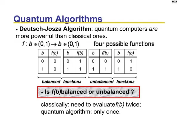
Quantum algorithms for SAT • Unstructured search • Multi-level unstructured search • Hogg’s algorithm • Adiabatic evolution
Unstructured search • Don’t use any knowledge of the problem’s structure; just pass in an assignment and ask “does this satisfy the expression?” • Well-known that you can find a satisfying assignment in O(1.42n) tests of satisfiability using Grover’s algorithm • The other quantum algorithms given here don’t do much better...
Multi-level unstructured search • Idea: perform a Grover search on a subset of the variables, then nest another search within the subspace of those variables that satisfies the expression • for 3-SAT, optimal “nesting level” is ~2/3 of the variables • can think of it as a natural quantum analogue of the DPLL algorithm • Results in an average case O(1.27n) query complexity for 3-SAT • worse than the square root of the best classical algorithm • could this be because expressions are very sensitive to the values of all the variables they contain? • Due to Cerf, Grover & Williams1.
Multi-level search example • Let’s solve (a v b) ^ (a v ¬c) ^ (¬a v b) ^ (a v c) • First, search in the space of (a, b); ie. find the satisfying assignments to (a v b) ^ (¬a v b) • This will give us a superposition |0a1b> + |1a1b> • Now search for a satisfying assignment to the original expression in this space • ending up with a (correct) superposition |1a1b0c>+|1a1b1c>
Hogg’s algorithm1 • Works in a similar way to Grover’s algorithm • in fact, Grover’s algorithm is a special case of it • Starts with a superposition over all assignments, then combines phase rotations Pt (based on the number of conflicts in a given assignment) with “mixing” matrices Mt: • |jend> = MnPn...M1P1|+> • These matrices are heuristically parametrised, and change over the course of the algorithm, becoming closer to the identity
Hogg’s algorithm (2) • Phase matrix (problem-dependent):Pii = eiπ K c(i) • where K changes throughout the run and c(i) is the number of conflicts in assignment i • compare Grover phase oracle Pii = -(-1f(i) ) • Mixing matrix (problem-independent):M = Hxn * T * Hxn [ Tii = eiπ L w(i) ] • where L changes throughout the run and w(i) is the Hamming weight of the binary string i • compare Grover diffusion Tii = -(-1(δi1)) • Values Mab in mixing matrix are only dependent on distance(a, b) • Values Pii in phase matrix are only dependent on number of conflicts in assignment i
Performance of Hogg’s algorithm • 1-SAT can be solved in 1 step with this algorithm • the number of conflicts in a 1-SAT assignment is the same as its distance from the solution • so we can choose our mixing matrix cleverly to destroy those assignments with >0 conflicts • For k-SAT, the number of conflicts provides a rapidly worsening estimate of the distance; we have to use heuristics to try to adjust the estimate • No rigorous worst-case analysis done, but simulation on (small) hard random instances of 3-SAT suggests an average case query complexity of O(1.05n)
Adiabatic evolution • Uses the quantum adiabatic theorem • Idea: start in the ground state of a known Hamiltonian, and continuously evolve to the unknown ground state of a “solution” Hamiltonian • The solution Hamiltonian is set up so its lowest energy eigenstate is the state with no conflicts (ie. the solution) • No rigorous analysis of its power has been made, but it’s known that problem instances exist that take exponential time (e.g. van Dam et al1) • these rely on a very large local minimum, and a hard-to-find global minimum • Due to Farhi et al2
Lower bounds for these algorithms • Proving lower bounds on time complexity is a bit tricky • One way we can do it for quantum algorithms is to consider query complexity • All of the algorithms mentioned here use oracles – black boxes which give us the answer to a question • If we can put a bound on the minimum number of calls to these oracles, this gives us an idea of the time complexity of the algorithms
Oracle models in SAT (1) • These quantum algorithms use (implicitly or otherwise) the following oracles: • “Black box” • Grover’s algorithm, multi-level Grover search f(x,E) 1 if x satisfies E 0 if x doesn’t x
Oracle models in SAT (2) • “Conflict counting” • Hogg’s algorithm, adiabatic algorithm f(x, E) The number of clauses in E that x doesn’t satisfy x
Oracle models in SAT (3) • Another obvious oracle is “clause satisfaction” • not used by any algorithms so far... f(x,c,E) 1 if x satisfies clause #c of E 0 if x doesn’t x
Lower bounds for oracle models • We consider bounds in the number of calls to these oracles – aka query complexity • Adversary method used: • consider multiple instances of the problem – i.e. multiple oracles – that are somehow “close” but different • show a limit on the amount any two instances can be distinguished with one oracle call • work out how many oracle calls are needed to distinguish them all • Several different formulations of the method • all known formulations have been shown to be equivalent1
Geometric adversary method • Summed over a set of N oracles, consider the largest possible overlap |xG> of an input |x> with the “good” states – ie. ones for which the oracle returns 1 • intuitively, the “best” value of |x> to input for any instance of the problem will produce the largest overlap • Can show that T2 ≥ N / ∑ || |xG>||2 • proof omitted
Lower bounds for oracle models (2) • Unstructured search is well-known to have a lower bound of W(2n/2) queries • This implies that the multi-level search should have the same worst-case lower bound, as it uses the same oracle • To put a bound on the other oracle models, we pick instances of SAT such that they essentially reduce down to unstructured search; i.e. so that the more powerful oracles are no help to us
Lower bound for the “conflict counting” oracle • We consider a set of 2n instances of SAT, each of which has a single and different satisfying assignment • Each instance has n clauses, varying in length from 1 to n variables • Set the clauses up so none of them “overlap” – i.e. cause conflicts with more than one assignment • The number of conflicts will then be 1 for every assignment, bar the satisfying assignment: the oracle becomes no more powerful than unstructured search • So we can show the minimum query complexity is W(2n/2)
Example expression used a ^ (¬a v b) ^ (¬a v ¬b v c) 000 001 010 011 100 101 110 111 Each assignment satisfies all but one clause
Lower bound for the “clause satisfaction” oracle • A similar approach. But this time, we need more clauses • Consider a set of 2n expressions which have different, unique satisfying assignments. Each expression has 2n clauses, and each clause of each expression contains all n variables • Can then show a bound of W(2n/2) queries, extensible to W(sqrt(m)), where m is the number of clauses • Considerably weaker! We need exponential input size to show an exponential lower bound
Example expression used (a v b v c) ^ (a v b v ¬c) ^ (a v ¬ b v c) ^ (a v ¬ b v ¬ c) ^ (¬ a v b v c) ^ (¬ a v b v ¬ c) ^ (¬ a v ¬ b v c) 000 001 010 011 100 101 110 111
Do these results extend to k-SAT? • No! van Dam et al1 have shown that, for 3-SAT, an algorithm using the conflict counting oracle can recover the input in O(n3) calls to the oracle • I’ve extended this to k-SAT to show that the input can be recovered in O(nk) calls • Idea behind this: once you know about the number of conflicts in all the assignments of Hamming weight k or less, you can work out the number of conflicts for all other assignments without needing to call the oracle again
Conclusion • SAT has been known for 50 years, but classical algorithms to solve it are still improving • Quantum algorithms haven’t beaten the performance of classical ones by much – if at all • Thinking about the oracle models we use – implicitly or otherwise – gives us clues to how we should develop quantum algorithms • It looks like no algorithm can solve SAT quickly without “looking inside” the clauses • It’s also clear that we can’t prove any lower bounds for k-SAT using these restricted oracle methods