INF 5300 - 30.3.2016 Detecting good features for tracking Anne Schistad Solberg
INF 5300 - 30.3.2016 Detecting good features for tracking Anne Schistad Solberg. Finding the correspondence between two images What are good features to match? Points? Edges? Lines?. Curriculum. Chapter 4 in Szeliski, with a focus on 4.1 Point-based features

INF 5300 - 30.3.2016 Detecting good features for tracking Anne Schistad Solberg
E N D
Presentation Transcript
INF 5300 - 30.3.2016Detecting good features for trackingAnne Schistad Solberg • Finding the correspondence between two images • What are good features to match? • Points? • Edges? • Lines? INF 5300
Curriculum • Chapter 4 in Szeliski, with a focus on 4.1 Point-based features • Recommended additional reading on SIFT features: • Distinctive Image Features from Scale-Invariant Keypoints by D. Lowe, International Journal of Computer Vision, 20,2,pp.91-110, 2004.
Goal of this lecture • Consider two images containing partly the the same objects but at different times or from different views. • What type of features are best for recognizing similar object parts in different images? • Features should work on different scales and rotations. • These features will later be used to find the match between the images. • This chapter is also linked to chapter 6 which we will cover in a later lecture. • This is useful for e.g. • Tracking an object in time • Mosaicking or stitching images • Constructing 3D models • Automatic image registration
Image matching • How do we compute the correspondence/geometric transform between these images? • Extract good features for matching (this lecture) • Estimating geometrical transforms for matching (later lecture) • In INF 2310 we picked points to match manually, now we want to find them automatically. • by Diva Sian • by swashford
What type of features are good? • Point-like features? • Region-based features? • Line-based features? • Edge-based features?
Point-based features • Point-based features should represent a set of special locations in an image, e.g. landmarks or keypoints. • Two main categories of methods for matching these keypoints (more next week): • Find points in an image that can be easily tracked, e.g. using correlation or least-squares matching. • Given one feature, track this feature in a local area in the next frame • Most useful when the motion is small • Find features in all images and match them based on local appearance. • Most useful for larger motion or stitching.
Four steps in feature matching • Feature extraction • Search for characteristic locations that define unique motion • Feature description • Select a suitable descriptor that is easy to match • Feature matching • Efficient search for matching candidates in other images • Feature tracking • Search a small neighborhood around the given location • An alternative to step 3. • The two first steps will be the focus today.
Point-based features • Point-based features should highlight landmarks or points of special characteristics in the image. • They are normally used for establishing correspondence between image pairs. • What kind of locations in these images do you think are useful? INF 5300
Feature detection • Goal: search the image for locations that are likely to be easy to match in a different image. • What characterizes the regions? How unique is a location? • Texture? • Homogeneity? • Contrast? • Variance? INF 5300
Feature detection – similarity criterion • A simple matching criterion: summed squared difference between two subimages: • I0 and I1 are the two images, u=(u,v) the displacement vector, and w(x) a spatially varying weight function. • For simplicity, the 2D image is indexed using a single index xi. • Check how stable a given location is (with a position change u)in the first image (self-similarity) by computing the summed square difference (SSD) function: • Note: the book calls this autocorrelation, but it is not equivalent to autocorrelation. 3 2 1 3 2 1 INF 5300
Feature detection: the math • Consider shifting the window W by ∆u=(u,v) • how do the pixels in W change? • E is based on the L2 norm which is relatively slow to minimize. • We want to modify E to allow faster computation. • If ∆u is small, we can do a first-order Taylor series expansion of E. • W
Feature detection: gradient tensor A • The matrix A is called the gradient tensor: • It is formed by the horizontal and vertical gradients. • If a location xi is unique, it will have large variations in S in all directions. • The elements of A is the summed horisontal/vertical gradients: • W
Information in the tensor matrix A • The matrix A carries information about the degree of orientation of the location of a patch. • A is called a tensor matrix and is formed by outer products of the gradients in the x- and y-direction, (Ix and Iy), convolved with a weighting function w to get a pixel-based estimate. • How is you intuition of the gradients: • In a homogeneous area? • Along a line? • Across a line? • On a corner? INF 5300
Information in the tensor matrix A • Eigenvector decomposition of A gives two eigenvalues, max and min. • The first eigenvector will point in the direction of maximum variance of the gradient • The smallest eigenvalue carries information about variance perpendicular to this (in 2D). • If max ≈ 0 and min ≈ 0 then this pixel has no features of interest • If min ≈ 0 and max has a large value, then an edge is found • If min has a large value then a corner/interest point is found ( max will be even larger) • High gradient in the direction of maximal change • If there is one dominant direction, min will be much smaller than max. • A high value of min means that the gradient changes much in both directions, so this can be a good keypoint. INF 5300
Feature detection: Harris corner detector • Harris and Stephens (1988) proposed an alternative criterion computed from the tensor matrix A (=0.06 is often used): • Other alternatives are e.g. the harmonic mean: • The difference between these criteria is how the eigenvalues are blended together. INF 5300
Adaptive non-maximal suppression (ANMS) • Points with high values of the criterion tend to be close together. • Suppress neighboring points by only detecting points that are local maxima AND significantly larger than all neighbors with radius r. INF 5300
Feature detection algorithm • Compute the gradients Ix and Iy , using a robust Derivative-of-Gaussian kernel (hint: convolve a Sobel x and y with a Gaussian). A simple Sobel can also be used, will be more noisy. • The scale used to compute the gradients is called the local scale. • Form Ix2, IxIy, and Iy2 • Smooth Ix2, IxIy, and Iy2 by a larger Gaussian and form A from averaging in a local window. • Compute either the smallest eigenvalue or the Harris corner detector measure from A. • Find local maxima above a certain threshold. • Use Adaptive non-maximal suppression (ANMS) to improve the distribution of feature points across the image. INF 5300
Examples Largest eigenvalue INF 5300
Harris operator Smallest eigenvalue INF 5300
We note that the first eigenvalue gives information about major edges. • The second eigenvalue gives information about other features, like corners or other areas with conflicting directions. • The Harris operator combines the eigenvalues. • It is apparent that we need to threshold the images and find local maxima in a robust way. • How did we supress local minima in the Canny edge detector?? INF 5300
Comparing points detected with or without suppressing weak points (ANMS) INF 5300
So now we have a method to detect locations of keypoints. • We also want invariance to • Scale • Robust keypoints can be at different scales • Orientation INF 5300
Rotation invariance • To match features in a rotated image, we want the feature descriptor (next stage) to be rotation invariant. • Option 1: use rotation-invariant feature descriptors. • Option 2: estimate the locally dominant orientation and create a rotated patch to compute features from. INF 5300
How do we estimate the local orientation? • The gradient direction is often noisy. • Many ways to robustify it: • Direction from eigenvector of gradient tensor matrix • Filter the the gradients gx, gy and gxy and form the gradient tensor matrix T. Compute the direction as the direction of the dominant eigenvector of T. For a robust estimate: • Smooth in a small window before gradient computation • Smooth the gradients in a larger window before computing the direction. • Angle histogram • Group the gradient directions for all pixels in a window weighted by magnitude together into a histogram with 36 bins. • Find all peaks in the histogram with 80% of maximum (allowing more than one dominant direction at some locations). INF 5300
How do we get scale invariance? • Goal: Find keypoint locations that are invariant to scale changes. • Solution 1: • Create a image pyramid and compute features at each level in the pyramid. • At which level in the pyramid should we do the matching on? Different scales might have different characteristic features. • Solution 2: • Extract features that are stable both in location AND scale. • SIFT features (Lowe 2004) is the most popular approach of such features. INF 5300
Scale-invariant features (SIFT) • See Distinctive Image Features from Scale-Invariant Keypoints by D. Lowe, International Journal of Computer Vision, 20,2,pp.91-110, 2004. • Invariant to scale and rotation, and robust to many affine transforms. • Scale-space: search at various scales using a continuous function of scale known as scale-space. To achieve this a Gaussian function must be used. • Main components: • Scale-space extrema detection – search over all scales and locations. • Keypoint localization – including determining the best scale. • Orientation assignment – find dominant directions. • Keypoint descriptor - local image gradients at the selected scale, transformed relative to local orientation. INF 5300
Definition of scale space • For a given image f(x,y), its linear (Gaussian) scale-space representation is a family of derived signals L(x,y,t) defined by the convolution of f(x,y) with the two-dimensional Gaussian kernel g(x,y,t) such that L(x,y,y)=G(x,y,t)*f(x,y) • This definition of works for a continuum of scales t , but typically only a finite discrete set of levels in the scale-space representation would be actually considered. • The scale parameter is the variance of the Gaussian filter As t increases, is the result of smoothing with a larger and larger filter, thereby removing more and more of the details which the image contains. • Why a Gaussian filter? • Sevaral derivations have shown that a Gaussian kernel is the best choice to assure that new structures must not be created when going from a fine scale to any coarser scale. The kernel is linear, shift invariant, preserved local maxima, and has scale- and rotation-invariance INF 5300
SIFT: 1. Scale-space extrema • The scale space is defined as the function L(x,y,) • The input image is I(x,y) • A Gaussian filter is applied at different scales L(x,y,) = G(x,y,)* I(x,y,). is the scale. • The Gaussian filter is: • Scale-space extrema are detected from the points (x,y;s) in 3D scale-space (x,y,s) at which the scale-normalized Laplacian assumes local extrema with respect to space and scale. • The scale-normalized Laplacian is normalized with respect to the scale level in scale-space and is defined as • This is an efficient approximation of a Laplacian of Gaussian, normalized to scale . Lowe (2004) uses =1.6. (For derivation of this see Marr & Hildreth 1980 DOI: 10.1098/rspb.1980.0020 ) INF 5300
SIFT: 1. Scale-space extrema • In practise, it is faster to approximate the Laplacian of Gaussian with a difference of Gaussian, normalized to scale . Lowe (2004) uses =1.6. (For derivation of this see Marr & Hildreth 1980 DOI: 10.1098/rspb.1980.0020 ) • Compute keypoints in scale space by difference-of-Gaussian (DOG), where the difference is between two nearby scales separated by a constant k: • The DOG includes a normalization and can be written: • In detailed experimental comparisons, Mikolajczyk (2002) found that the maxima and minima of DOG produce the most stable image features compared to a range of other possible image functions, such as the gradient, Hessian, or Harris corner function INF 5300
SIFT: 1. Scale-space extrema illustration • For each octave of scale: • Convolve the image with Gaussians of different scale. • Compute Difference of Gaussians for adjacent Gaussians on a given octave. • The next octave is down-sampled by a factor of 2. • Each octave is divided into an integer number of scales s, s+3 images in each octave is selected. INF 5300
SIFT 2 : accurate extrema detection • First step in minimum/maximum detection: compare the value of D(x,y,) to its 26 neighbors in this scale, and the scale above and below. • The candidate locations afterthisprocedurearethenchecked for fitaccording to location, scale, and principalcurvature. • This is explainedonthenext slide. INF 5300
SIFT 2: extrema detection • Consider a Taylor series expansion of the scale-space function D(x,y,) around sample point x • The location of the extreme point is found by take the derivative of D(x) and setting it to zero: • It is computed by differences of neighboring sample points, yielding a 3x3 linear system. • The value of D at the extreme point is useful for suppressing extrema with low contrast, |D|<0.03 are suppressed. INF 5300
SIFT 2: eliminating edge response based on curvature • Since points on an edge are not very stable, such points need to be eliminated. • This is done using the curvature, computed from the Hessian matrix of D. • The eigenvalues of H are proportation to principal curvatures of D. Consider the ratio between the eigenvalues and . A good criteria is to only keep the points where • r=10 is often used. INF 5300
SIFT 3: computing orientation • To normalize for the orientation of the keypoints, we need to estimate the orientation. The feature descriptors (next step) will then be computed relative to this orientation. • They used the gradient magnitude m(x,y) and direction (x,y) to do this (L is a Gaussian smoothed image at the scale where the keypoints were found). • Then, they computed histograms of the gradient direction, weighted by gradient magnitude. The histograms are formed from points in the neighborhood of a keypoint. • 36 bins covers the 360 degrees of possible orientations. • In this histogram, the highest peak, and other peaks with height 80% of max are found. If a localization has multiple peaks, it can have more than 1 orientation. • WHY are locations with more than one orientation important? INF 5300
Feature descriptors • Which features should we extract from the key points? • These features will later be used for matching to establish the motion between two images. • How is a good match computed (more in chapter 8)? • Sum of squared differences in a region? • Correlation? • The local appearance of a feature will often change in orientation and scale (this should be utilized e.g. by extracting the local scale and orientation and then use this scale (or a coarser one) in the matching). INF 5300
SIFT 4: feature extraction stage • Given • Keypoint locations • Scale • Orientation for each keypoint • What type of features should be used for recognition/matching? • Intensity features? Use correlation as match? • Gradient features? • Similar to our visual system. SIFT uses gradient features. INF 5300
SIFT: feature extraction stage • Select the level of the Gaussian pyramid where the keypoints were identified. • Main idea: use histograms of gradient direction computed in a neighborhood as features. • Compute the gradient magnitude and direction at each point in a 16x16 window around each keypoint. Gradients should be rotated relative to the assigned orientation. • Weight the gradient magnitude by a Gaussian function. Each vector represents the gradient magnitude and direction. The circle illustrates the Gaussian window. INF 5300
SIFT 4: feature extraction stage • Form a gradient orientation histogram for each 4x4 quadrant using 8 directional bins. The value in each bin is the sum of the gradient magnitudes in the 4x4 window. • Use trilinear interpolation of the gradient magnitude to distribute the gradient information into neighboring cells. • This results in 128 (4x4*8) non-negative values which are the raw SIFT-features. • Further normalize the vector for illumination changes and threshold extreme values. This illustration shows a 2x2 descriptor array and not 4x4 INF 5300
Variations of SIFT • PCA-SIFT: compute x- and y-gradients in a 39x39 patch, resulting in 3042 features. Use PCA to reduce this to 36 features. • Gradient location-orientation histogram (GLOH): use a log-polar binning of gradient histograms, then PCA. • Steerable filters: combinations of DoG-filters of edge- and corner-like filters. INF 5300
Feature matching • Matching is divided into: • Define a matching strategy to compute the correspondence between two images. • Using efficient algorithms and data structures for fast matching (we will not go into details on this). • Matching can be used in different settings: • Compute the correspondende between two partly overlapping images (= stitching). • Most key points are likely to find a match in the two images. • Match an object from a training data set with an unknown scene (e.g. for object detection). • Finding a match might be unlikely INF 5300
Computing the match • Assume that the features are normalized so we can measure distances using Euclidean distance. • We have a list of keypoints features from the two images.Given a keypoint in image A, compute the similarity (=distance) between this point and all keypoints in image B. • Set a threshold to the maximum allowed distance and compute matches according to this. • Quantify the accuracy of matching in terms of: • TP: true positive: number of correct matches • FN: false negative: matches that were not correctly detected. • FP: false positive: proposed matches that are incorrect. • TN: true negative: non-matches that were correctly rejected. INF 5300
Evaluating the results How can we measure the performance of a feature matcher? 50 75 200 feature distance
Performance ratios • True positive rate (TPR) • TPR = TP/(TP+FN) • False positive rate (FPR) • FPR = FP/(FP+TN) • Positive predictive value (PPV) • PPV = TP/(TP+FP) • Accuracy (ACC) • ACC = (TP+TN)/(TP+FN+FP+TN) • Challenge: accuracy depends on the threshold for a correct match! INF 5300
Evaluating the results How can we measure the performance of a feature matcher? # true positives # matching features (positives) # false positives # unmatched features (negatives) ROC curve (“Receiver Operator Characteristic”) 1 0.7 truepositiverate 0 1 false positive rate 0.1 ROC Curves • Generated by counting # current/incorrect matches, for different threholds • Want to maximize area under the curve (AUC) • Useful for comparing different feature matching methods
SIFT: feature matching • Compute the distance from each keypoint in image A to the closest neighbor in image B. • We need to discard matches if they are not good as not all keypoints will be found in both images. • A good criteria is to compare the distance between the closest neighbor to the distance to the second-closest neighbor. • A good match will have the closest neighbor should be much closer than the second-closest neighbor. • Reject a point if closest-neighbor/second-closest-neighbor >0.8. INF 5300
Feature tracking - introduction • Feature tracking is a alternative to feature matching. • Idea: detect features in image 1, then track each of these features in image 2. • This is often used in video applications where the motion is assumed to be small. • Is the motion assumed small: • Can the grey levels change? Use e.g. cross-correlation as a similarity measure. • Large motion: • Can appearance changes happen? • More on this in a later lecture. INF 5300
Edge-based features • Edge-based features can be more useful than point-based features in 3D or e.g. when we have occlusion. • Edge-points often need to be grouped into curves or countours. • An edge is considered an area with rapid intensity variation. • Consider a gray-level image as a 3D landscape where the gray level is the height. Areas with high gradient are areas with steep slopes, computed by the gradient • J will point in the direction of the steepest ascent. • Taking the derivative is prone to noise, so we normally apply smoothing first/or in combination by combining the edge detector with a Gaussian. INF 5300
Edge detection using Gaussian filters • Gradient of a smoothed image: • Derivative of Gaussian filter: • Remember that the second derivative (Laplacian) carries information about the exact location of the edge: • The edge locations are locations where the Laplacian changes sign (called zero crossing). • Edge pixels can then be linked together based on both magnitude and direction. INF 5300
Scale selection in edge detection • is the scale parameter. • It should be determined based on noise characteristics of the image, but also knowledge about the average object size in the image. • A multi-scale approach is often used. • After edge detection, we can apply all methods for robust boundary representation from INF 4300 to describe the contour. They can be normalized to handle different types of invariance. INF 5300