Progress in Linear Programming Based Branch-and-Bound Algorithms
Progress in Linear Programming Based Branch-and-Bound Algorithms. Andrew Miller University of Wisconsin. Objectives. To discuss what techniques are being used to solve mixed integer programs in practice

Progress in Linear Programming Based Branch-and-Bound Algorithms
E N D
Presentation Transcript
Progress in Linear Programming Based Branch-and-Bound Algorithms Andrew Miller University of Wisconsin
Objectives • To discuss what techniques are being used to solve mixed integer programs in practice • To discuss what can be accomplished with commercial mixed integer optimizers and modeling languages
Outline • Introduction and linear programming based branch-and-bound • Branch-and-cut and branch-and-price
Why Use MIP ? • Indivisible commodities • Binary choices • Logical relations • Start up or fixed costs • Economies of scale • Combinatorial modeling
Tremendous increase of the use of MIPs in the last decade Large-scale MIPs are solvable (provably good solutions) on PCs with commercially available software Applicability
Transportation planning and operations Facility location Production scheduling Supply-chain management Many others Recent Applications
Aircraft arrival slot allocation at American. Network optimization used to allocate arrival slots of canceled flights, leading to reduced delays, translates into direct annual operating cost savings of $5.2M (1991) Optimizing airline scheduling of planes and crews. Delta's Cold Start solves its fleet assignment with expected savings of $300M over three years (1994) Transportation planning and operations
Base closing in Germany (US Department of Defense). 0-1 IP used to determine base closures and optimal stationing plan for US troops in Europe after force reductions, annual savings of up to $58M (1996) Facility location
Fiber-optic cable manufacturing (AT&T). MIP models select fibers and schedule cable production resulting in more efficient use of fibers and fewer delays in customer orders (1998) Production scheduling
Global supply chain management (Digital). MIP used to design production, distribution and vendor network so as to minimize cost of production and distribution times, saved $100M (1995) Restructuring the supply chain (Proctor and Gamble). MIP is used to help restructure the supply chain (1997) Supply-chain management
LP Based Branch and Bound • Implicit enumeration tree • At every node, an LP relaxation is solved • Upper bounds come from LP solutions; lower bounds come from MIP feasible solutions
LP Based Branch and Bound Initialization zip=-, xip= List empty? xip optimal Choose problem Solve LPzlp,xlp If infeasible, then fathom If zlp zip, then fathom If xlp integral, then zipzlp,xip xlp and fathom Branch
How to improve performance? 1. Faster computer 2. Faster linear programming optimizer 3. Smaller zlp 4. Larger zip 5. Improved branching 6. Smaller linear programs
Most MIPs have many correct formulations, but while one formulation may be easy to solve, another may be very hard to solve Failure to solve a MIP may not be the fault of the algorithm, but the result of a “bad” formulation Smaller size formulations (number of variables and constraints) may not be better and can be much worse Formulations
xij: fraction of demand of client i satisfied from depot j yj: 1 if depot j is open 0 otherwise Uncapacitated Facility Location
Uncapacitated Facility Location • Question: Can we do this automatically ?
Parallel Machine Scheduling xij:1 if job j is scheduled on machine i C: makespan
Parallel Machine Scheduling • Problem: Symmetry Swapping assignments to two machines gives the exact same solution! • Solution: Remove symmetry from solution
Branching Strategies • Variable selection • Node selection
Variable Selection • Variable dichotomy: ( xj = xj + fj ) xj xj xj xj • GOAL: Select a variable that improves the upper bound the most
Prediction Methods • Estimation methods • Lower bounding methods
Estimation Methods Pseudocosts • Pj+ Per unit change in objective function value when the variable j is rounded up • Pj- Per unit change in objective function value when the variable j is rounded down Estimates • Dj+ = Pj+ (1 - fj ) • Dj- = Pj- fj
Lower Bounding • Lj+ Lower bound on the per unit change in objective function value when the variable j is rounded up • Lj- Lower bound on the per unit change in objective function value when the variable j is rounded down
Combining Estimation and Lower Bounding • Estimation provides global information • Lower bounding provides local information • Compute parameters a priori • Compute parameters dynamically
Using Predictors • How to select branching variable ?
Node Selection GOAL: (1) Find good feasible solution (2) Prove optimality
Node Selection Methods • static • estimate-based • two-phase • backtracking
Static Methods • best-first (best-bound) • advantages • minimizes number of evaluated nodes • disadvantages • high memory requirements • high node evaluation times
Static Methods • depth-first • advantages • minimizes memory requirements • low node evaluation times • high chance of finding feasible solutions quickly • disadvantages • large search trees
Estimate-based Methods • best projection
Estimate-based Methods • best estimate Note: Does not require zbest
Two-phase Methods • Phase I: Find good feasible solution • Phase II: Prove optimality
Two-phase Methods • Phase I: Depth-first • Phase II: Best-first
Two-phase Methods • Phase I: Best estimate • Phase II: Maximize Percentage Error
Backtracking Methods • Go depth-first as often as possible • If zlp E, then depth-first • If zlp E, then best-first or best-estimate
Preprocessing Detecting infeasibility Detecting redundancy Improving bounds Preprocessing and Probing
Detecting Infeasibility • If z > bi, then infeasible • Approximation • Simple Approximation
Detecting Infeasibility 3x1 - 4x2 + 2x3 6 -3x1 + 4x2 - 2x3 -6 -3 + 0 - 2 = -5 > -6 infeasible
Tentatively fixing a variable at one of its bounds and examining the consequences Three activities Fixing variables Improving coefficients Identifying logical implications Probing
Fixing Variables • If zk > bi, then infeasible • Conclusion: xk 1 or xk = 0 • Simple Approximation
Fixing Variables Probing x2 = 1 3x1 - 4x2 + 2x3 2 -3x1 + 4x2 - 2x3 -2 -3 + 4 - 2 = -1 > -2 infeasible x2 = 0
xj = 0, fixes xk = 0 xkxj fixes xk = 1 1- xkxj xj = 1, fixes xk = 0 xk 1 - xj fixes xk = 1 1- xk 1 - xj Identifying logical implications
Diving Heuristic Solve LP Infeasible? Give up Integral? Stop Analyze LP solution. Fix some variables. Round up or down some variables and fix them.