Combinatorial Auctions with a Black Box Model
Combinatorial Auctions with a Black Box Model. Noam Nisan Hebrew University, Jerusalem. Talk Structure. The “demand oracle” model for combinatorial auctions Definition Justification Complexity of combinatorial auctions Polynomial upper bound when a Walrasian equilibrium exists

Combinatorial Auctions with a Black Box Model
E N D
Presentation Transcript
Combinatorial Auctions with a Black Box Model Noam Nisan Hebrew University, Jerusalem
Talk Structure • The “demand oracle” model for combinatorial auctions • Definition • Justification • Complexity of combinatorial auctions • Polynomial upper bound when a Walrasian equilibrium exists • Exponential lower bound for the general case • Approximation algorithm for the general case • Results for classes of combinatorial auctions • Submodular valuations • Duplicate items • Procurement auctions
Combinatorial Auctions • N indivisible non-identical items for sale • m bidders compete for subsets of these items • Each bidder i has a valuation for each set of items: vi(S) = value that i assigns to acquiring the set S • vi is non-decreasing (“free disposal”) • vi() = 0 ״״״ • Objective: Find a partition (S1…Sm) of {1..N} that maximizes the social welfare: ivi(Si) • Issues: communication, allocation, strategies
Complements and Substitutes • vj() may have complements: vj(ST) > vj(S)+vj(T) for some S and T. • Extreme case: “single-minded bid” -- will only pay for a complete package -- pay p for the set S but pay nothing for anything else • vj() may have substitutes: vj(ST) < vj(S)+vj(T) for some disjoint S and T. • Extreme case: “unit demand bid” -- will pay for at most a single item – the price may depend on the item
Routing as a Combinatorial Auction Bidder A Destination Bidder B Bidder C • Each bidder wants to buy some path to the destination • Each link is an item
The FCC Spectrum Auctions • The FCC auctions spectrum licenses for many geographic regions and various frequency bands • These auctions have raised billions of dollars • The value of a license to a bidder depends on the other licenses it holds • Currently licenses are sold in a simultaneous auction • USA Congress mandated that the next spectrum auction be made combinatorial. 3.1-3.2GHz 3.1-3.2GHz 3.2-3.3GHz 3.2-3.3GHz 3.3-3.4GHz 3.1-3.2GHz 3.2-3.3GHz 3.1-3.2GHz 3.1-3.2GHz 3.2-3.3GHz 3.2-3.3GHz 3.3-3.4GHz
How to handle the valuation functions vi ? • Economics approach: vector of numbers • Ignores exponential communication costs • Ignores allocation complexity (NP-hardness) • CS approach: Represent in some bidding language • Language restricts the space of valuations • Results depend on the bidding language • Impossibility results are not concrete: NP-completeness • This talk: Black-box (oracle) approach • The valuation is represented by a black-box that can answer specified queries about the valuation function. The mechanism can only ask these queries. • Computational efficiency == few (polynomial) queries • Computational inefficiency == many (exponential) queries
Demand Oracle • Valuation Oracle Query: • Input: subset S • Output:v(S) • Demand Oracle Query: • Input:N item prices: p1…pN • Output:D(p1…pN) -- Demand at these prices. I.e. the set S that maximizes v(S)-jS pj • A Demand oracle can simulate a valuation oracle in a polynomial number of queries (polynomial in the number of items and the number of bits of precision of the output) • A Demand oracle may be exponentially more powerful than the valuation oracle
Simulating a Valuation Oracle Algorithm for computing v(S) using a valuation oracle: marginal-valuation(j,S): For all goods iS set pi=0; for all other goods set pi= Perform a binary search on pj to find lowest value with D(p1…pN)=S v(S): Initialize: result=0 For all goods jS do result result + marginal-valuation( j, {iS | i<j } )
Justification of the Demand Oracle Model • Can easily be used by mechanisms: • Natural for several classes of mechanisms • Strong enough for everything I looked at • Myopic bidders will answer queries truthfully • Can be efficiently computed for bidding languages: • Single package bids • XOR bids • OR bids on disjoint sets of items • Paths in networks • Lower bounds apply also to any oracle • Oracle model combines computation and communication points of view in a concrete abstract setting
A Natural Tatonnement Process Demange&Gale&Sotomayor Initialize item prices: p1=0, p2=0, …, pN=0 Repeat: For each bidder i query Di(p1…pN) For each item j that is demanded by more than a single bidder do pj pj+ Until: all items are demanded by at most a single bidder Theorem: If valuations are “gross substitutes” then this finds an allocation that is N close to optimal.Kelso&Crawford • This is a special case that has a Walrasian Equilibrium • A combinatorial auction has a Walrasian equilibrium if the “relaxed LP” has an integral solution. Bikhchandani&Mamer
Walrasian Equilibrium Definition: A set of prices p1…pN and an allocation D1…Dm is called a Walrasian equilibrium if for every bidder i, Di=Di(p1…pN). First Welfare Theorem: For any Walrasian equilibrium, D1…Dm is an optimal allocation. Proof: For any other allocation S1…Sm: Note: Optimality is also over fractional allocations. Corollary: the appropriate LP has integral solutions.
Solving the Linear Program The Dual LP Minimize: . Subject to: • For each i, S: • For each i, j: An infeasible solution can be detected using demand oracles: for each bidder i enough to test for S=Di(p1…pN) Ellipsoid method can find solution in polynomial time (despite exponential number of constraints). The Primal LP Maximize: . Subject to: • For each item j: • For each bidder i: • For each i, S:
The General Case Theorem: In the worst case, an exponential (in N) number of queries are needed (even for 2 bidders, even with 0/1 valuations, and even without requiring any type of equilibrium) Nisan&Segal Proof: Definition:Answers(A,v1,v2) Is the sequence of answers for the queries that algorithm A asked on bids v1,v2 • For every valuation v of bidder 1, with v({1…N}) =1, we will define a valuation v* for bidder 2, and show, Main Lemma: If A always finds optimal allocations, then for every uv, we have Answers(A,v,v*) Answers(A,u,u*). Corollary: (number of answers) (number of valuations) (total length of answer sequence) (representation length of valuation) = exponential number of queries is exponential.
Proof of Main Lemma Definition:v*(S)=1-v( ) Facts: • For every v, S, we have v(S)+v*( ) = 1 • For every u(S)>v(S) we have u(S)+v*( ) > 1 v(S)+u*( ) < 1 Cut-and-paste lemma: If Answers(A,u,u*)=Answers(A,v,v*) then also Answers(A,u,v*)=Answers(A,v,u*) • Proof: the query answers will keep being the same in all 4 cases Corollary: If u v, then Answers(A,u,u*) Answers(A,v,v*) • Proof: the optimal S for (u,v*) is sub-optimal for (v,u*)
Remarks on Lower Bound • A general communication lower bound • Applies also for “non-deterministic” communication • Applies even if valuations of sets are 0,1 • When valuations are continues the message space must have exponential dimension • May be viewed as a lower bound for number of “prices”
Approximation Algorithm For each bidder i find set Si that maximizes vi(Si)/|Si| (binary search) For all i, in decreasing order of vi(Si)/|Si|, do If no item jSi was previously allocated then Allocate Si to i If (total value of solution found) < vi({1…N}) for some i then Ignore current solution and allocate everything toi Theorem: This gives a -approximation Theorem: Any algorithm that gives a better than a ratio requires an exponential number of queries.
Proof of upper bound Case 1: Allocating everything to a single bidder provides an approximation to within a factor of Case 2: Take the optimal allocation, and remove sets whose size is at least . Since the valuation of each such set is at most of the total, we have removed at most ¼ of the total valuation. Let T1…Tk be the remaining sets. Claim 1: for each bidder i, vi(Si)/|Si|vi(Ti)/|Ti| Definition: for bidders i with Si= define b(i) to be first bidder that was allocated an item in Si. Claim 2: for each b there are at most |Sb| values i such that b=b(i). Claim 3: for bidders i with Si=, vb(i)(Sb(i))/|Sb(i)|vi(Ti)/|Ti| Claims 1+2+3 Since we get that
Lower bound – approximate packing Input: collections C1…Cm of subsets of {1…N} Output: distinguish between the following extreme cases • There exist disjoint sets S1C1 … Sm Cm (m-packing) • Any two sets SiCiand SjCj (ij) intersect (no 2-packing) Model:m-party communication (number-in-hand) Theorem: Requires bits of communication Proof: via reduction to approximate-disjointness
Approximate Disjointness Input: binary strings s1…sm of length t each Output: distinguish between the following extreme cases • There exists an index r such that for all i,si[r]=1 (NO) • For every index r at most a single i, si[r]=1 (YES) Model:m-party communication (number-in-hand) Theorem: Requires bits of communication Alon&Matias&Szegedy Proof: (of bound) Radhakrishnan&Srinavasan • Total number of YES instances = • Every YES-box B1*...*Bmcontains no NO-instances, thus for every index r there exists i such that for all siBi, si[r]=0 ==> Total number of YES instances in YES-box ==> Total number of YES-boxes
The Reduction Input: binary strings s1…sm of length t each Output: collections C1…Cm of subsets of {1…N} such that • exists r where for all i,si[r]=1 IFF exist disjoint sets S1C1 … SmCm • every r at most a single i, si[r]=1 IFF every SiCiand SjCj intersect Construction: • Fix a set of partitions P1…Pt of {1…N}, (Where each Pr=(Pr1…Prm)). • Take Ci={Pri | si[r]=1} • We need that each two parts of different partitions intersect • Probabilistic construction of P1…Pt : • For fixed r,s,i,j: • Thus t can be taken to be
Submodular Valuations Definition: v is submodular if for all S, T: v(S T) + v(S T) v(S) + v(T) Equivalently: v is submodular iff it has decreasing marginal valuations: S T ==> v(T a) - v(T) v(S a) - v(S) Algorithm: Lehman&Lehman&Nisan Initialize, for all bidders i, Si= For every item j do Find i that maximizes vi(SiU j) – vi(Si) Si Si U j Theorem: If all valuations are submodular then this is a 2-approximation. Theorem: An exponential number of queries are needed to find an exact solution (or a (1+1/(4N))-approximation) even for submodular valuations. Nisan&Segal
Auctions with Duplicate Items Bartal&Gonen&Nisan • Assume that there are k units of each good. • Each bidder wants at most one from each good type – i.e. vi() is still a functions of sets (rather than multi-sets). • Assumption (for now): vmin < vi({1…N}) < vmax Online Algorithm: Initialize item prices: p1=…=pN = vmin / (2kN) For all bidders i: Si Di(p1…pN) For all items jSi do Observation: No item is allocated > k times Theorem: This gives a approximation.
Proof of approximation Ratio Notation: • OPT=( T1 … TN) is the optimal solution. • ALG=(S1…SN) is the output of the algorithm. • Pj* is the final value of Pj. Claim 1: Corollary 1: Claim 2: Last bidder that received item j, paid for it Pj* / Corollary 2: We conclude by summing k *(corollary 2) + (corollary 1), and taking into account that
Incentive Compatibility Definition: A mechanism is incentive compatible if truth is a dominating strategy for all players. For combinatorial auctions it means that for any vi, v`i, v-i: • Si and piare i’s allocation and payment on input (vi,v-i) • S`i and p`i are i’s allocation and payment on input (v`i,v-i) Theorem: the online algorithm is incentive compatible (when players actually pay the prices that they were faced with.)
Characterization of Incentive Compatible CAs Theorem: A direct revelation mechanism is incentive compatible if and only if for every bidder i and every vector of bids of the other players v-i it: • Fixes a price pS for every possible allocation S to bidder i, and whenever bidder i isallocated S, his payment is pS. (Note that pS does not depend on vi). • For every vi, it allocates to i the set S that maximizes the value ofvi(S)-pS. Proof: • Payment depends only on set won, which is optimal • If payment pS depends on bid vi manipulation helps • If S is not optimal then i would optimize by lying
Removing the assumption on vmin, vmax • The algorithm only used vmin for price initialization and could instead use any lower bound on |OPT| • We could simply use maxi vi({1…N}) instead – this gets rid of the vmin/vmax term. • Incentive compatibility would be destroyed only for the bidder that determined this maximum • We can fix this by changing the allocation rule for this bidder only to use the second highest price instead of the highest price. • Two things become worse: • An extra unit of each good may be allocated • The approximation ratio becomes worse • Thus our approximation ratio is
Procurement Auctions • vi(S) now specifies supplier i’s cost for supplying S • The goal is to minimize the total cost for a partition {Si} • Demand oracle should return set that maximizes the supplier’s benefit: iS pi – v(S) Algorithm:(Basically Lovasz) Initialize: for all suppliers i, Si= While Ui Si {1…N} do Find i and that minimize vi(S)/|S| Si Si U S Theorem:If all valuations are sub-additive then this is a ln(N) approximation. Theorem: Getting a better than ln(N)/ln(4) approximation requires exponential queries.