Download
1 / 30
300 likes | 528 Vues
Numerical Modeling of Flow and Transport Processes Calculating Laminar Natural Convection H eat Transfer Coefficient on a horizontal cylinder using Comsol Software Joseph Addy 31103196 Supervised by Professor Manfred Koch. Motivation Introduction to COMSOL Software

E N D
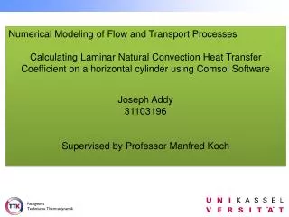
Numerical Modeling of Flow and Transport Processes Calculating Laminar Natural Convection Heat Transfer Coefficient on a horizontal cylinder using Comsol Software Joseph Addy 31103196 Supervised by Professor Manfred Koch
Motivation • Introduction to COMSOL Software • Natural Convection and Governing Equations • Boundary and Initial conditions for Problem description • Comsol Implementation • Conclusion Table of Contents
Simulation is fast and delivers local and global information in details, for instance, the velocity field or pressure distribution in a pipe. • Simulation provides approximate solution to real problems and also cheaper. • Numerical modeling provides general knowledge and understanding for the mode of operation of products and processes Motivation
COMSOL Multiphysics software is a powerful finite element (FEM), partial differential equation (PDE) solution engine. The software has eight add-on modules that expand the capabilities in the following application areas: • AC/DC Module • Acoustics Module • Chemical Engineering • Earth Science • Heat transfer • MEMS (microelectromechanical systems) • RF • Structural Mechanics • The Multiphysics has CAD Import Module and the Material Library as supporting software COMSOL Software
COMSOL Software Multiphysics implies multiple branches of physics can be applied within each model. Comsol facilitates all steps in the modeling begining with your geometry, meshing , specifying your physics ( subdomain and boundary conditions), solving and then visualizing your results. Comsol can solve problems in 1D, 2D, 3D and axial symmetries in 1 and 2D
Comsol Multiphysics provides the power to simulate and model systems that involve • Mass transport including migration in the concentrated solutions • Laminar, turbulent , multiphase and porous media flows • Energy transport and thermodynamic systems Comsol Multiphysics
From the application modes one chooses the type of problem to be solved and from the space dimension, the type of dimension. Comsol software
Natural Convection refers to convection in which the fluid is driven thermally; that is , fluid motion is driven by buoyancy, as a result of density gradients that is induced in the fluid whether it is heated or cooled. The velocities induced by the density gradients are small and therefore the natural heat transfer coefficient are lower than forced convection. The governing differential equations for natural convection are based on the conservation of mass, momentum and thermal energy. The density difference in natural convection is driven by a temperature difference and known as Boussinesq aprroximation( where the density is assumed to depend linearly on the temperature). Natural Convection (free convection)
The conservation mass, momentum and energy equations in differential forms respectively Governing Equations The left part of the momentum and energy equations consist of the convective and local part of the derivative
For incompressible Newtonian fluid: the density was held constant and the shear stress is proportional to the velocity gradient. Governing Equations Principle of mass conservation Principle of conservation of momentum for incompressible fluid. The second law of Newton states that mass multiplied by acceleration is equal to the sum of body and surface forces acting on the body
Governing Equations Dissipation , source and sink are neglected Energy cannot be created nor destroyed, but can be transformed from one state to another ρ: density cp: specific heat capacity η: dynamic viscosity P: pressure f: volume force sp(T.D): dissipation energy T: temperature u: velocity in x direction v: velocity in y direction div: vector differential operator
In natural convection problems, the density difference is driven by the temperature variation and the term relating to the fluid property is known as volumetric thermal expansion coefficient at a given pressure. The induced velocity increases with the temperature difference and the thermal expansion coefficient. Governing Equations
Considering the similarity for dimensionless parameters to obtain the boundary layer aprroximation . We define nondimensional variables and introduce them into the conservation mass, momentum and thermal energy equations by substitution. Governing Equations
Governing Equations The free stream velocity is substituted into momentum and energy equations respectively
The correlating parameters on the right-hand side of the conservation equations are direct consequences of buoyancy forces and they are identical. Governing Equations The Grashof number Gr characterizes the importance of buoyancy forces relative to viscous forces. It is similar to Reynold`s number in forced convection . The solution for a heat transfer coefficient h in natural convection is determind using Rayleigh number Ra, the geometry of the problem and Nusselt number Nu. The Rayleigh number is a product of the Grashof and Prandtl numbers. The Rayleigh number determines whether the free convection is laminar or turbulent at the critical boundary.
4 The momentum and energy equations are inherently coupled since the temperature appears in the momentum equation and the velocity in the energy equation. Geometry description with boundary and initial conditions 3 5 7 6 1 2
The Navier-Stokes equation is coupled with the heat equation From the Applications Mode , choose Comsol Multiphysics Add heat transfer to Fluid dynamics Comsol Implementation
In the option builder the physical quantities used in the computation are expressed using the film temperature except the thermal expansion coefficient which depends on the free stream temperature Comsol Implementation
Comsol Implementation The subdomain settings allow us to specify physical properties of the fluid,initial conditions and mode of heat transfer. The boundary condition considers what is happening at the boundaries of the geometry.
Generating a mesh to solve the problem with overly dense mesh covering specific boundary conditions on the left hand side of the geometry Comsol Implementation
From the computation the Normal total heat flux is needed for the calculation of the average heat transfer coefficient. Normal Total Heat Flux
The Nusselt number is a function of the Rayleigh`s number, therfore the heat transfer coefficient depend on both values. • An analytical computation was carried out in order to compare the results. The simulation shows a high field of accuracy with the literature. The computed value from the literature for the heat transfer coefficient is 7.5W/(m^2*K), while the Comsol simulation was 7.8W/(m^2*K). Comsol is easy to use, but demands a high understanding of computation fluid dynamics. Conclusion
Heat transfer : Karl Stephan • Heat transfer: Gregory Nellis and Sanford Klein • Matlab for poisson equation: Professor Koch • Multiphysics modeling Comsol: Roger W. Pryor • Stanford University Lecture: Prof.Barba Lorenza References