Understanding Transport Processes in Surface Waters: Emission, Immission, and Mass Balance

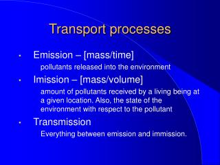
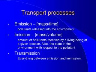
1. Transport processes • Emission – [mass/time] pollutants released into the environment • Imission – [mass/volume] amount of pollutants received by a living being at a given location. Also, the state of the environment with respect to the pollutant • Transmission Everything between emission and immission.

2. Transport processes What is a transport process? • Describes the fate of any material in the environment • The continuous steps of transportation, reactions and interactions which happen to the pollutants • It determines the concentration-distribution of the observed material in time and in space • Transmission

3. Transport processes Transport processes include: • Physical transportation due to the movement of the medium • Advection • Diffusion and dispersion • Physical, chemical, biochemical conversion processes: • Settling • Ad- and desorption • Reactions • Degradation, decomposition

4. Transport processes What is our aim? • Defend our values • Decrease the immission by controlling the emission – EFFORT, MONEY! • Describe transport processes

5. Transport processes Important concepts: • State variable: concentration, density, temperature… • Conservative material: no reactions, no settling • Non-conservative material: opposite, realistic • Flow processes: 3D, u(x,y,z,t), h(x,y,z,t), V(x,y,z,t),… • Steady state: du/dt=0, dC/dt=0,… • Homogeneous distribution – totally mixed reactor

6. Transport processes This presentation deals only with transport processes in surface waters. So the transporting medium is water. Classical water quality state variables are: • Dissolved oxygen (DO) • Organic material - biochemical oxygen demand (BOD) • Nutrients – N-, P-forms (NO3-N, PO4-P,…) • Suspended solids (SS) • Algae

7. OUT (2) (1) Controlling surface V IN Mass balance General mass balance equation: • Expresses the conversation of mass! • Differential equations IN – OUT + SOURCES – SINKS = CHANGE We work with mass fluxes [g/s]

8. Mass balance By solving the general mass balance equation we can describe the transport processes for a given substance. Solution: • Analytical • Numerical Discretization: • Temporal • Spatial • Boundary, initial conditions: • Geometrical DATA • Hydrologic DATA • Water quality DATA • Simplifications: • Temporal – steady-state • Spatial – 2D, 1D • Other

9. Simplified case I. IN – OUT + SOURCES – SINKS = CHANGE Assumptions: • Steady state • Conservative material Solution • IN=OUT • SOURCES=0, SINKS=0 • CHANGE=0

10.  H vs Simplified case II. Assumptions: • Steady state – Q(t), E(t) are constants, dC(t)/dt=0 • Non-conservative, settling material (vs) • Prismatic river bed – A, B, H are constants • 1D A ~ B·H [m2]

11. (1) (2) Q Q Av Simplified case II. x IN: OUT: C(x) is linear (assumption) LOSS: settled matter

12.  v vs The calculation Simplified case II. If x=O C=Co Exponential decrease

13. E E=q·c emission Dilutionratio Determination of C0 value Simplified case II. Cbgbackgroundconcentration C0 concentration under the inlet Q 1D – Complete mixing (two water mixing with each other) Increment:

14. Dilution Sedimentation The solution Simplified case II. Transmission coefficient Conservative matter!!!

16. The general situation • Unsteady • Inhomogeneous • Non-conservative • 3D General transport equation: Advection-Dispersion Equation (ADE)

17. Advection-dispersion Equation • Can be derived from the mass balance. • Expresses the temporal and spatial changes of the observed state variable • It’s solution is the concentration-distribution over time • Differential equation Change due to diffusion or dispersion Change due to conversion processes Change in concentration with time Change due to advection = + +

18. v CONVECTION Molecular diffusion DIFFUSION

19.   c1 c2  x Fick’sLaw Molecular diffusion • c1 c2 separated tanks • open valve • equalization and mixing • (Brown-movement) • depends on temperature Mass flux (kg/s) through area unit D - molecular diffusion coefficient [m2/s]

20. dz dy dx Mass balance equation IN: conv + diff OUT: conv + diff x direction IN OUT • convection • diffusion CHANGE

21. dz dy dx Mass balance equation IN: conv + diff OUT: conv + diff x direction

22. Convection Diffusion Mass balance equation Convection: transfering Diffusion: spreading If D(x) = const. in x direction Convection - Diffusion 1D Equation The other directions are similar

23. Mass balance equation x, y, z directions (3D): Convection: The water particles with different concentrations of pollutant move according to their differing flow velocity Diffusion: The adjacentwater particlesmix with each other, which causes the equalization of concentration D – molecular diffusion coefficient material specific, water: 10-4 cm2/s space independent slow mixing and equalization

24. v*deviation, pulsation 0 Turbulence • Laminar flow: ordered with parallel flow lines • Turbulent flow: disordered, random (flow and direction) because of surface roughness (friction) → causes intensive mixing • Natural streams: always turbulent v (c)  average t T Time step of the turbulence We usually can use the average only!!

25. Turbulent transport description Convection:v·c [ kg/m2·s ] 0 ? 0

26. v turbulent diffusion molecular diffusion Turbulent diffusion X direction (the other are similar) Analogy with Fick’s Law → the original transport equation does not change, only the D parameter Dtx, Dty, Dtz>> D Depends on the direction Function of the velocity space!!!

27. 3D transport equation in turbulent flow Dx = D + Dtx, Dy = D + Dty, Dz = D + Dtz Temporal averaging (T) Convection Diffusion Turbulent diffusion Stochastic fluctuations of the flow velocity (pulsations) Diffusive process in mathematical sense (~ Fick’s Law) Convective transport!!! (temporal differences)

28. x H v z Spatial simplifications (2D) - Dispersion Velocity depth profile Depth averaged flow velocity Depth Integration (3D2D) v 0 After the expansion of the convectiv part (v ·c) in x direction Turbulent dispersion (~ diffusion)

29. 2D transport equation in turbulent flow (depth averaged) Dx*, Dy*turbulentdispersion coefficients in 2D equation Depth averaging (H) 1D transport equation in turbulent flow (cross-section av.) Dx**turbulentdispersion coefficient in 1D equation Cross-section averaging (A)

30. v Turbulent dispersion Convectiv transport arising from the spatial differences of the velocity profile (faster and slower particles compared to the average) In the 2D and 1D equations only! Dispersion coefficient: a function of the velocity space (hydraulic parameters, channel geometry) Dx* = Ddx+ Dtx + DDy* = Ddy+ Dty+ D Dx** = Ddxx + Ddx+ Dtx + D Dx*, Dy* >> Dx Dx** >> Dx* In case of more irregular channel and higher depth or larger cross-section area its value is bigger Also present in laminar flow

31. 1. settling 2. settling X2 X - efficiency ( 0 , 1 ) X1 FOLYÓ E - BOD5 emission E2 E1 LAKE 2 3 Industrial use bath (CR3) (O2 standard, CR2) 1 REGIONAL PROBLEM: COST EFFICIENT SOLUTION • Immission standard  C2 + a12E1X1  CR2 a - coefficient of transport  C3 + a13E1X1 + a23E2X2  CR3 C2, C3 – present state (monitor)

32. 1 xU  C2 + a12E1X1  CR2  C3 + a13E1X1 + a23E2X2  CR3 xL xL xU 1 • FIRST STEP x2 x1 • SECOND STEP WHAT WAS NOT APPLIED? min [K1(X1) + K2(X2)] FUNCTION WE NEED min [k1X1 + k2X2] LINEAR TYPE • SOLUTION IS THE COST FUNCTION OK?

33. 1 xU xL xL xU 1 • CONDITION (1) and (2) x2 • “RELATIVE” IMPORTANCE • ENGINEER AND RESEARCHER • OUTLET • TECHNOLOGICAL LIMIT • MINIMUM NEED x1 • “EVEN” STRATEGY • AFTER THIS: DEFINE COSTS AND FACTOR TRANSPORT