Discretization in space and time. Transport processes
530 likes | 754 Vues
Discretization in space and time. Transport processes. Earth-System Modeling (A. Paul and M. Schulz). Schedule. Schedule. Suggested reading.

Discretization in space and time. Transport processes
E N D
Presentation Transcript
Discretization in space and time.Transport processes Earth-System Modeling (A. Paul and M. Schulz)
Suggested reading • Washington, Warren M. and Parkinson, Claire L.: An Introduction to Three-Dimensional Climate Modeling. 2nd edition. University Science Books, Sausalito, California, 2005. • Chapter 4 (e.g. Sections on “Finite Differences” and “Finite Differencing in two dimensions”). • In German: Stocker, Thomas (2008), Einführung in die Klimamodellierung (lecture notes, 146 pp), http://www.climate.unibe.ch/~stocker/papers/skript08EKM.pdf. • Chapter 3, e.g. Sections 3.1, 3.4, 3.5, 3.8. In the following, I mainly adhere to the notation of the lecture notes by T. Stocker.
Atmosphere and ocean transport matter and energy by winds and currents.
Transport processes • Advection • associated with fluid flow that transports matter and energy • Diffusion • stochastic process • Convection • caused by unstable stratification (heavy fluid overlies light fluid)
Transport processes are crucial in the climate system • Heat transport in the atmosphere • Salt transport and spreading of tracers in the ocean
Advection • Fluid (gas, air, water) flows with velocity u(x,t)through control area A(x) • Transported quantitiy(mass, energy, momentum, tracer) is given as concentration C(x,t), i.e . refers to a unit volume
Advection One-dimensional flow along x axis (Figure 3.1 from Stocker 2008)
During time intervalt, let the flow cover a volume • Then the total quantity transported is: Note: The symbol D (as used to denote the time step Dt or the grid step Dx) indicates a small but finite (non-zero) quantity.
The flow of the quantity, relative to the area A and time interval t, is called a flux density:
In three dimensions, the advective flux density of a scalar quantity C in a flow with velocity u(x,t) is • The flux density is a vector in the direction of the flow.
Quantity Formula General scalar Mass Heat flux Salt flux x-component of momentum Advective flux density
State variables • Many variables can be thought of as a “concentration“ or “property per unit volume“. • Fluxes then have dimensions of “property per unit time and area”.
Diffusion One-dimensional flow along x-axis (Figure 3.2 from Stocker 2004). x-axis is divided in cells of width Dx. Each cell contains molecules in disordered motion, corresponding to a temperature T.
Describe the random motion of the molecules by a probability p for a jump of one particle from cell i to cell i+1. • Let rbe the number of molecules per cell (number density).
The number of particles jumping from cell i to the right is: • The number of particles jumping from cell i+1 to the left is:
The (mass) flux at the boundary between cells i and i+1 is given by or
In the limit the diffusive flux density of mass becomes
K is the diffusion coefficient in units of m2 s-1. It parameterizes processes at the non-resolved molecular scale. • Net diffusive fluxes only occur if the density or concentration gradient is non-zero.
In three dimensions, the diffusive flux density of a scalar quantity C is
Where: isotropic diffusion coefficient (scalar) gradient operator, turns scalar C(x,y,z) into vector that points into the direction of steepest ascent of the surface given by z=C(x,y,z)
Convection • Convection occurs when potential energy is released by the flow. • E.g. cold air overlying warm air (in atmospheric boundary layer) leads to diffusive heat flux until all potential energy is released and the temperature difference is removed
Convection also occurs in the ocean in areas of large winter cooling or sea-ice formation. • Parameterized using an explicit mass- and energy-conserving mixing scheme or large, stability-dependent diffusion coefficients.
Advection equation • Consider a concentration C in a fixed control volume Spatially varying flux density in one dimension (Figure 3.3 from Stocker 2008).
Conservation of mass or amount is described by: inflow outflow Devide byV = Ax :
Introduce partial derivatives: partial derivative of the concentration C(x,t) with respect to time t, at a fixed point in space x. partial derivative of the concentration C(x,t) with respect to location x (i.e., concentration gradient), at a fixed instant in time x.
Change order of fluxes: With finite-volume method, this minus sign appears “naturally”. Flux form of one-dimensional advection equation. Take limit Divergence of flux in x-direction
For discretizing the advection-diffusion-equation, I generally prefer to start from the flux form, which in combination with the finite-volume method ensures the conservation of any scalar variable C in a natural manner.
Numerical solution of the one-dimensional advection equation • Spatial discretization: • Temporal discretization: • Solution at space-time grid points:
In most climate models, only two or three time levels are retained to save computer memory: • two time levels: present future • three time levels: past present future
To solve the one-dimensional advection equation numerically, we need to replace the temporal and spatial derivatives by finite-difference representations.
Discretization in time • Approximate (partial) derivative with respect to time t by ratio of finite differences: Euler forward or Forward in Time (FT) Euler backward or Backward in Time (CT) Centered in Time (CT)
Insert into one-dimensional advection equation and solve for future time level, e.g.: Euler forward or Forward in Time (FT) Centered in Time (CT)
Discretization in space • Approximate (partial) derivative with respect to location x by first recovering the flux form: Outflow – inflow at the present time level . • For example, the “centered-in-time” scheme becomes:
Then express fluxes Fi,in terms of the concentrations Ci,and the flow velocity ui: Where, for example: Upstream or upwind (“Backward in Space”, BS) Or: Centered in Space (CS)
Consider the concentration Ci,in a grid cell centered at the grid point with x-coordinate xi, and a constant flow velocity ui-1=ui=u0 that is directed to the right: ui-1 ui Ci+1 Ci-1 Ci x direction xi xi+1 xi-1 • To estimate the incoming flux Fi-1, , • the “upstream” or “upwind“ scheme uses the concentration Ci-1,to the left, while • the “centered-in-space” scheme uses the average of the concentrations Ci-1,and Ci,.
(+1)·t ·t (-1)·t i·x CTCS (centered-in-time, centered-in-space) or “leap-frog” scheme on space-time grid. The information at two previous time levels is used to predict the solution at the future time level (Figure 3.5 from Stocker 2008).
Stability criterion • Courant-Friedrich-Levy criterion for stable solution with centered differences : “No transport faster than one grid cell per timestep” or Large current velocities (jet stream in the atmosphere, western boundary currents in the ocean) require small time steps.
How fast is ocean transport? • Western boundary currents transport warm and saline water from tropics to middle latitudes • Examples: Kuroshio, Gulf Stream, Brazil Current, Agulhas Current • Strongest current velocities near 2 m s-1 • Deep western boundary currents flow from north to south at a depth of 2-3 km. • Maximum flow velocity in its core (2.5 km depth) 20 cm s-1
Finite differences: advantages • Positive-definite schemes possible (e.g. “Prather scheme”) • Adaptable to complex geometry (e.g. coastlines, bottom topography)
Finite differences: disadvantages • Convergence of meridians requires small time step
Other methods • Finite elements (mostly used in engineering applications) • Spectral method (used in many atmospheric general circulation models)
Spectral method • Global atmospheric fields can be represented in terms of spherical basis functions • Similar to the use of trigonometric functions such as sines or cosines See Washington and Parkonson (1986), Chapter 4, pp. 18.
Fourier theorem • Example: vibrating string, stretched along an x-axis and fixed at both ends, with the left end at x = 0 and the right end at x = l.
Fourier theorem • The actual shape of the vibrating string can always be represented as an infinite series of eigenvector basis functions: where
Fourier theorem The two lowest modes of a vibrating string with fixed end points [Figure 4.5 from Washington and Parkinson (1986)].
Spectral method: advantages • Easy and exact spatial differentiation • Natural description of planetary waves in unbounded domain • Homogenous resolution on a sphere • Advection without dispersion
Spectral method: disadvantages • Transformations become computationally inefficient at high resolution • For any truncated basis function expansion, there is overshooting and undershooting (Gibbs phenomenon) • occurs near steep gradients • yields negative values of mass and humidity • makes representation of mountain ranges or ice sheets difficult