Enhancing Wildfire Forecasting with Space-Time Point Processes: A New Approach

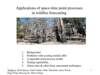
1. Applications of space-time point processes in wildfire forecasting Background Problems with existing models (BI) A separable point process model Testing separability Alarm rates & other basic assessment techniques Thanks to: Herb Spitzer, Frank Vidales, Mike Takeshida, James Woods, Roger Peng, Haiyong Xu, Maria Chang.

2. Los Angeles County wildfires, 1960-2000

3. Background • Brief History. • 1907: LA County Fire Dept. • 1953: Serious wildfire suppression. • 1972/1978: National Fire Danger Rating System. (Deeming et al. 1972, Rothermel 1972, Bradshaw et al. 1983) • 1976: Remote Access Weather Stations (RAWS). • Damages. • 2003: 738,000 acres; 3600 homes; 26 lives. (Oct 24 - Nov 2: 700,000 acres; 3300 homes; 20 lives) • Bel Air 1961: 6,000 acres; $30 million. • Clampitt 1970: 107,000 acres; $7.4 million.

6. NFDRS’s Burning Index (BI): • Uses daily weather variables, drought index, and • vegetation info. Human interactions excluded.

7. Some BI equations: (From Pyne et al., 1996:) Rate of spread: R = IRx (1 + fw+ fs) / (rbe Qig). Oven-dry bulk density: rb = w0/d. Reaction Intensity: IR = G’ wn h hMhs. Effective heating number: e = exp(-138/s). Optimum reaction velocity: G’ = G’max (b/ bop)A exp[A(1- b / bop)]. Maximum reaction velocity: G’max = s1.5 (495 + 0.0594 s1.5) -1. Optimum packing ratios: bop = 3.348 s -0.8189. A = 133 s -0.7913. Moisture damping coef.: hM = 1 - 259 Mf /Mx + 5.11 (Mf /Mx)2 - 3.52 (Mf /Mx)3. Mineral damping coef.: hs = 0.174 Se-0.19 (max = 1.0). Propagating flux ratio: x = (192 + 0.2595 s)-1 exp[(0.792 + 0.681 s0.5)(b + 0.1)]. Wind factors: sw = CUB (b/bop)-E. C = 7.47 exp(-0.133 s0.55). B = 0.02526 s0.54. E = 0.715 exp(-3.59 x 10-4 s). Net fuel loading: wn = w0 (1 - ST). Heat of preignition: Qig = 250 + 1116 Mf. Slope factor: fs = 5.275 b -0.3(tan f)2. Packing ratio: b = rb / rp.

8. On the Predictive Value of Fire Danger Indices: • From Day 1 (05/24/05) of Toronto workshop: • Robert McAlpine: “[DFOSS] works very well.” • David Martell: “To me, they work like a charm.” • Mike Wotton: “The Indices are well-correlated with fuel moisture and fire activity over a wide variety of fuel types.” • Larry Bradshaw: “[BI is a] good characterization of fire season.” • Evidence? • FPI: Haines et al. 1983 Simard 1987 Preisler 2005 Mandallaz and Ye 1997 (Eur/Can), Viegas et al. 1999 (Eur/Can), Garcia Diez et al. 1999 (DFR), Cruz et al. 2003 (Can). • Spread: Rothermel (1991), Turner and Romme (1994), and others.

9. Some obvious problems with BI: • Too additive: too low when all variables are med/high risk. • Low correlation with wildfire. • Corr(BI, area burned) = 0.09 • Corr(BI, # of fires) = 0.13 • Corr(BI, area per fire) = 0.076 • Corr(date, area burned) = 0.06 • Corr(windspeed, area burned) = 0.159 • Too high in Winter (esp Dec and Jan) • Too low in Fall (esp Sept and Oct)

14. Some obvious problems with BI: • Too additive: too high for low wind/medium RH, Misses high RH/medium wind. (same for temp/wind). • Low correlation with wildfire. • Corr(BI, area burned) = 0.09 • Corr(BI, # of fires) = 0.13 • Corr(BI, area per fire) = 0.076 • Corr(date, area burned) = 0.06 • Corr(windspeed, area burned) = 0.159 • Too high in Winter (esp Dec and Jan) • Too low in Fall (esp Sept and Oct)

16. More problems with BI: • Low correlation with wildfire. • Corr(BI, area burned) = 0.09 • Corr(BI, # of fires) = 0.13 • Corr(BI, area per fire) = 0.076 • Corr(date, area burned) = 0.06 • Corr(windspeed, area burned) = 0.159 • Too high in Winter (esp Dec and Jan) • Too low in Fall (esp Sept and Oct)

17. r = 0.16 (sq m)

18. More problems with BI: • Low correlation with wildfire. • Corr(BI, area burned) = 0.09 • Corr(BI, # of fires) = 0.13 • Corr(BI, area per fire) = 0.076 • Corr(date, area burned) = 0.06 • Corr(windspeed, area burned) = 0.159 • Too high in Winter (esp Dec and Jan) • Too low in Fall (esp Sept and Oct)

21. Constructing a Point Process Model as an Alternative to BI…. Definition: A point process N is a Z+-valued random measure N(A) = Number of points in the set A.

22. More Definitions: • Simple: N({x}) = 0 or 1 for all x, almost surely. (No overlapping pts.) • Orderly: N(t, t+ D)/D ---->p 0, for each t. • Stationary: The joint distribution of {N(A1+u), …, N(Ak+u)} does not depend on u.

23. Intensities (rates) and Compensators • -------------x-x-----------x----------- ----------x---x--------------x------ • 0 t- t t+ T • Consider the case where the points are observed in time only. • N[t,u] = # of pts between times t and u. • Overall rate: m(t) = limDt -> 0 E{N[t, t+Dt)} / Dt. • Conditional intensity: l(t) = limDt -> 0 E{N[t, t+Dt) | Ht} / Dt, where Ht = history of N for all times before t. • If N is orderly, then l(t) = limDt -> 0 P{N[t, t+Dt) > 0 | Ht} / Dt.

24. Intensities (rates) and Compensators -------------x-x-----------x----------- ----------x---x--------------x------ 0 t- t t+ T These definitions extend to space and space-time: Conditional intensity: l(t,x) = limDt,Dx -> 0 E{N[t, t+Dt) x Bx,Dx | Ht} / DtDx, where Ht = history of N for all times before t, and Bx,Dx is a ball around x of size Dx. The conditional intensity uniquely characterizes the distribution of a simple process. Suggests modeling l. e.g. Model l(t,x) as a function of BI on day t, interpolating between stations at x1, x2, …, xk using kernel smoothing:

27. Model Construction • -- Some Important Variables: • Relative Humidity, Windspeed, Precipitation, Aggregated rainfall • over previous 60 days, Temperature, Date. • -- Tapered Pareto size distribution g, smooth spatial background m. l(t,x,a) = b1exp{b2R(t) + b3W(t) + b4P(t)+ b5A(t;60) + b6T(t) + b7[b8 - D(t)]2} m(x) g(a). Two immediate questions: a) How do we fit a model like this? b) How can we test whether a separable model like this is appropriate for this dataset?

28. Conditional intensity l(t, x1, …, xk; q): [e.g. x1=location, x2 = size.] • Separability for Point Processes: • Say l is multiplicative in mark xj if l(t, x1, …, xk; q) = q0lj(t, xj; qj) l-j(t, x-j; q-j), where x-j = (x1,…,xj-1, xj+1,…,xk), same for q-j and l-j • If l~is multiplicative in xj^ and if one of these holds, then • qj, the partial MLE,= qj, the MLE: • S l-j(t, x-j; q-j) dm-j = g, for all q-j. • S lj(t, xj; qj) dmj = g, for all qj. ^~ • S lj(t, x; q) dm= S lj(t, xj; qj) dmj = g, for all q.

29. Individual Covariates: • Suppose l is multiplicative, and • lj(t,xj; qj) = f1[X(t,xj); b1] f2[Y(t,xj); b2]. • If H(x,y) = H1(x) H2(y), where for empirical d.f.s H,H1,H2, • and if thelog-likelihood is differentiable w.r.t. b1, • then the partial MLE of b1 = MLE of b1. (Note: not true for additive models!) • Suppose lis multiplicative and the jth component is additive: • lj(t,xj; qj) = f1[X(t,xj); b1] + f2[Y(t,xj); b2]. • If f1 and f2 are continuous and f2 is small: • S f2(Y; b2)2 / f1(X;~b1) dm / T ->p 0], • then the partial MLE b1 is consistent.

30. Impact • Model building. • Model evaluation / dimension reduction. • Excluded variables.

31. Model Construction l(t,x,a) = b1exp{b2R(t) + b3W(t) + b4P(t)+ b5A(t;60) + b6T(t) + b7[b8 - D(t)]2} m(x) g(a). Estimating each of these components separately might be somewhat reasonable, as a first attempt at least, if the interactions are not too extreme.

32. r = 0.16 (sq m)

33. Testing separability in marked point processes: Construct non-separable and separable kernel estimates of l by smoothing over all coordinates simultaneously or separately. Then compare these two estimates: (Schoenberg 2004) May also consider: S5 = mean absolute difference at the observed points. S6 = maximum absolute difference at observed points.

35. S3 seems to be most powerful for large-scale non-separability:

36. Testing Separability for Los Angeles County Wildfires:

37. r = 0.16 (sq m)

39. (sq m) (F)

42. Model Construction • Wildfire incidence seems roughly separable. (only area/date significant in separability test) • Tapered Pareto size distribution f, smooth spatial background m. [*] l(t,x,a) = b1exp{b2R(t) + b3W(t) + b4P(t)+ b5A(t;60) + b6T(t) + b7[b8 - D(t)]2} m(x) g(a). Compare with: [**] l(t,x,a) = b1exp{b2B(t)} m(x) g(a), where B = RH or BI. Relative AICs (Poisson - Model, so higher is better):

44. Comparison of Predictive Efficacy

45. One possible problem: human interactions. • …. but BI has been justified for decades based on its correlation with observed large wildfires (Mees & Chase, 1993; Andrews and Bradshaw, 1997). • Towards improved modeling • Time-since-fire (fuel age)

46. (years)

47. Towards improved modeling • Time-since-fire (fuel age) • Wind direction

50. Towards improved modeling • Time-since-fire (fuel age) • Wind direction • Land use, greenness, vegetation