Download
1 / 52
520 likes | 658 Vues
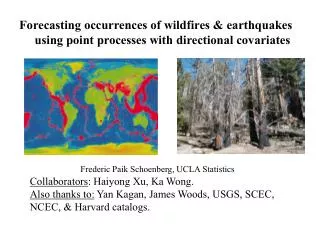
Forecasting occurrences of wildfires & earthquakes using point processes with directional covariates. Frederic Paik Schoenberg, UCLA Statistics Collaborators : Haiyong Xu, Ka Wong. Also thanks to: Yan Kagan, James Woods, USGS, SCEC, NCEC, & Harvard catalogs. Background

E N D
Forecasting occurrences of wildfires & earthquakes using point processes with directional covariates Frederic Paik Schoenberg, UCLA Statistics Collaborators: Haiyong Xu, Ka Wong. Also thanks to: Yan Kagan, James Woods, USGS, SCEC, NCEC, & Harvard catalogs.
Background Existing point process models for wildfires & earthquakes Problems, esp. wind & moment tensors Directional kernel direction & wind Using focal mechanisms in ETAS
Background • Brief History. • 1907: LA County Fire Dept. • 1953: Serious wildfire suppression. • 1972/1978: National Fire Danger Rating System. (Deeming et al. 1972, Rothermel 1972, Bradshaw et al. 1983) • Damages. • 2003: 738,000 acres; 3600 homes; 26 lives. (Oct 24 - Nov 2: 700,000 acres; 3300 homes; 20 lives) • Bel Air 1961: 6,000 acres; $30 million. • Clampitt 1970: 107,000 acres; $7.4 million.
Global Earthquake Data: • Local e.q. catalogs tend to have problems, esp. missing data. • 1977: Harvard (global) catalog created. • Considered the most complete. Errors best understood. • Harvard Catalog, 1/1/84 to 4/1/07 • Shallow events only (depth < 70km) • Mw 3.0+ • Only focal mechanism estimates of high or medium quality
2. Existing models for forecasting eqs & fires • NFDRS’s Burning Index (BI): • Uses daily weather variables, drought index, and • vegetation info. Human interactions excluded.
Some BI equations: (From Pyne et al., 1996:) Rate of spread: R = IRx (1 + fw+ fs) / (rbe Qig). Oven-dry bulk density: rb = w0/d. Reaction Intensity: IR = G’ wn h hMhs. Effective heating number: e = exp(-138/s). Optimum reaction velocity: G’ = G’max (b/ bop)A exp[A(1- b / bop)]. Maximum reaction velocity: G’max = s1.5 (495 + 0.0594 s1.5) -1. Optimum packing ratios: bop = 3.348 s -0.8189. A = 133 s -0.7913. Moisture damping coef.: hM = 1 - 259 Mf /Mx + 5.11 (Mf /Mx)2 - 3.52 (Mf /Mx)3. Mineral damping coef.: hs = 0.174 Se-0.19 (max = 1.0). Propagating flux ratio: x = (192 + 0.2595 s)-1 exp[(0.792 + 0.681 s0.5)(b + 0.1)]. Wind factors: sw = CUB (b/bop)-E. C = 7.47 exp(-0.133 s0.55). B = 0.02526 s0.54. E = 0.715 exp(-3.59 x 10⁻⁴ s). Net fuel loading: wn = w0 (1 - ST). Heat of preignition: Qig = 250 + 1116 Mf. Slope factor: fs = 5.275 b -0.3(tan f)2. Packing ratio: b = rb / rp.
Point Process Models • Conditional ratel(t, x1, …, xk; q): [e.g. x1=location, x2 = area.] • a non-neg. predictable process such that ∫ (dN -ldm) is a martingale. • Wildfire incidence seems roughly multiplicative. (only marginally significant in separability test) • Roughly exponential in relative humidity (RH), windspeed (W), precipitation (P), avg precip over prior 60 days (A), temperature (T), and date (D). • Tapered Pareto size distribution f, smooth spatial background m. l(t,x,a) = f(a) m(x) b1exp{b2R(t) + b3W(t) + b4P(t) + b5A(t) + b6T(t) + b7[b8 - D(t)]2} Or, split by season: l(t,x,a) = f(a) m(x) B1,i exp{b2,i R(t) + b3,i W(t) + b4,i P(t) + b5,i A(t) + b6,i T(t)}
Aftershock activity described by modified Omori Law: K/(t+c)p
3. Some problems with existing models • BI has low correlation with wildfire. • Corr(BI, area burned) = 0.09 • Corr(date, area burned) = 0.06 • Corr(windspeed, area burned) = 0.159 • Too high in Winter (esp Dec and Jan) • Too low in Fall (esp Sept and Oct)
3. Some problems with existing models, continued • Wildfires: no use of wind direction. • Santa Ana winds (from NE) typically hot & dry. • ETAS: no use of focal mechanisms. • Summary of principal direction of motion in an earthquake, as well as resulting stress changes and tension/pressure axes.
4. Directional kernel regression and wind: ∑i yi gk(q - qi) / ∑ gk(q - qi), using a circular kernel g, such as the von-Mises density gk(q) = exp{k cos(q)}/2p I0(k).
4. Directional kernel regression and wind: f(q) estimated via ∑i yi gk(q - qi) / ∑ gk(q - qi), using a circular kernel g, such as the von-Mises density gk(q) = exp{k cos(q)}/2p I0(k).
Distance to next event, in relation to nodal plane of prior event
In ETAS (Ogata 1998), l(t,x,m) = f(m)[m(x) + ∑i g(t-ti, x-xi, mi)], where f(m) is exponential, m(x) is estimated by kernel smoothing, and i.e. the spatial triggering component, in polar coordinates, has the form: g(r, q) = (r2 + d)q . Looking at inter-event distances in Southern California, as a function of the direction qi of the principal axis of the prior event, suggests: g(r, q; qi) = g1(r) g2(q - qi | r), where g1 is the tapered Pareto distribution, and g2 is the wrapped exponential.
tapered Pareto / wrapped exp. biv. normal (Ogata 1998) Cauchy/ ellipsoidal (Kagan 1996)
Thinned residuals: Data tapered Pareto / wrapped exp. Cauchy/ ellipsoidal (Kagan 1996) biv. normal (Ogata 1998)
Tapered pareto / wrapped exp. Cauchy / ellipsoidal
Cauchy/ ellipsoidal (Kagan 1996) biv. normal (Ogata 1998) tapered pareto / wrapped exp.
Conclusions: • The impact of directional variables on a scalar response can readily be summarized using directional kernel regression. • The resulting function can then be incorporated into point process models, to improve forecasting of the response variable. • Wildfires: wind direction is very significant, and models incorporating wind direction and other weather variables forecast about twice as well as the BI (which uses these same variables). • Earthquakes: focal mechanism estimates should be used to improve triggering functions in ETAS models.
On the Predictive Value of Fire Danger Indices: • From Day 1 of Toronto workshop (05/24/05): • Robert McAlpine: “[It] works very well.” • David Martell: “To me, they work like a charm.” • Mike Wotton: “The Indices are well-correlated with fuel moisture and fire activity over a wide variety of fuel types.” • Larry Bradshaw: “[BI is a] good characterization of fire season.” • Evidence? • FPI: Haines et al. 1983 Simard 1987 Preisler 2005 Mandallaz and Ye 1997 (Eur/Can), Viegas et al. 1999 (Eur/Can), Garcia Diez et al. 1999 (DFR), Cruz et al. 2003 (Can). • Spread: Rothermel (1991), Turner and Romme (1994), and others.


![The signs of the times(2) [earthquakes]](https://cdn1.slideserve.com/2296340/the-signs-of-the-times-2-earthquakes-dt.jpg)