
MTF Definition
E N D
Presentation Transcript
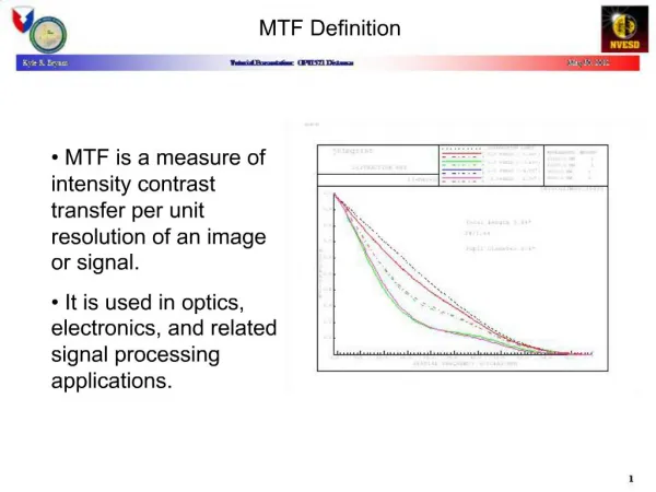
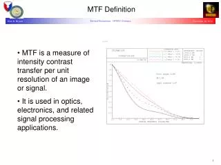
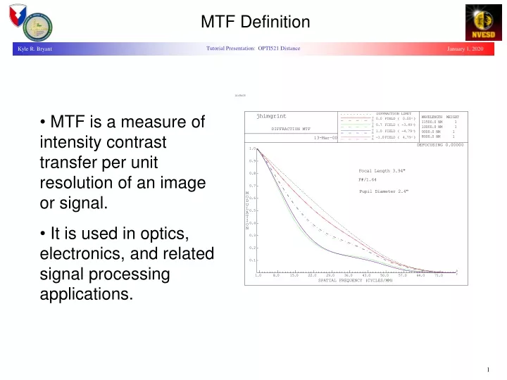
MTF Definition • MTF is a measure of intensity contrast transfer per unit resolution of an image or signal. • It is used in optics, electronics, and related signal processing applications.
Good Poor Imaging Task As spatial separation decreases, the “good” system maintains clear separation of point source images, while the “poor” system eventually can no longer distinguish them. MTF quantifies this phenomenon in terms of contrast between the center peak intensities versus intensity at their midpoint across a scale of separation distances. At large separations, even a poor system can completely resolve the two images. As separation decreases, only the good systems can still recognize separate sources.
Output Signal Imax Imin Original Signal One line pair Contrast Modulation: A Basic MTF Contrast Modulation is defined simply by averaging the difference of maximum and minimum transmitted intensities: “Spatial Frequency” typically implies an array of sine or bar targets at a given spacing, expressed in line-pairs-per-millimeter (lp/mm) or cylces -per-milliradian (cy/mrad)
Nyquist Sampling Theory Nyquist Theory: In order to achieve perfect reconstruction of an input signal which has a maximum spatial frequency "f" (the cutoff), sampling must occur at a rate of at least "2f". (Note: Phase is still an issue!) Input Waveform Input Waveform Sample Intervals in Phase Samples Out of Phase Sampled Output Sampled Output
Optical MTF Imaging optical systems perform sampling, with the maximum sample frequency determined by the “spot size” image of a perfect point source object (e.g., “Impulse Response”). A “perfect” optical system is limited in resolution by wavelength (l) dependent diffraction effects. Lens aberrations can only worsen performance. The MTF of an optical system is found by Fourier operations on the “spot size”, or Point Spread Function. Image Object For an Object source at infinity distance: For a Diffraction Limited Circular Aperture: Frequency Scale Conversion:
System MTF The MTF of cascaded optical assemblies is NOT equal to the product of component MTF’s! Why? Lenses transmit not just intensity, but wavefront phase as well, and hence aberrations in one lens can cancel those in another. MTF of cascaded objective lenses, detector, and displays may be multiplied for composite “System MTF”, with a component MTF measured at each intensity transfer point. Focal Plane Image Focal Plane Image MTFsystem¹ MTFLens1*MTFLens2 MTFsystem = MTFobjective*MTFdetector*MTFdisplay*MTFeyepiece*MTFeye
System MTF Example System MTF calculation: Freq. ObjLens FPA Display Eyepiece System cy/mrad MTF MTF MTF MTF MTF 1.0 0.9999 0.9999 0.9999 0.9999 0.99 2.0 0.90 0.99 0.99 0.90 0.79 3.0 0.85 0.98 0.92 0.88 0.67 For average human observers, MTF values around 0.05 are considered barely resolvable. If the above system MTF reached 0.05 at 10 cy/mrad, for example, then you can predict that a human observer couldidentify (6 cylce criteria) a 2.4 meter taget through this sensor at a maximum range (this is a coarse estimate!) of about
Measurement: Mathematical Functions 1. Measure the instensity profile ("spot size") Point Spread Function, or in 1D case, the Line Spread Function, with an optical instrument (not as easy as it sounds sometimes) 1 1 2 2 2 1 1 1 1 3 1 1 1 2 1 25 52 25 1 2 1 2 3 52 100 52 3 2 1 2 1 25 52 25 1 2 1 1 1 3 1 1 1 1 2 2 2 1 1 2. Calculate the modulus (absolute value) of the Fourier Transform of the PSF or LSF, cut out the foldover reflection, normalize to 1.0, and set the frequency scale based on cutoff calculation for n0as shown earlier. Discrete Fourier Transform: A typical MTF plot is really only one-dimensional (e.g., derived from the Line Spread Function. Hence, MTF's are typically plotted with curves for orthogonal Radial and Tangential orientations.
Differentiate Line Spread Edge Response Measurement: Knife Edge Knife Edge Measure of the Line Spread Function (LSF): 1. Drag a knife-edge across the focal plane of the optic to be tested and record the intensity 2. Calculating the derivative of this data gives us the LSF we are looking for so we can continue with MTF. 3. The discrete derivative sequence diof a sequence of numbers xi is easy: di = ||xi- xi+1|| (we want the absolute values here)