Dynamic trees (Steator and Tarjan 83)
290 likes | 315 Vues
This text introduces dynamic trees and the operations that can be performed on them, such as finding roots, adding and finding costs, linking and cutting, and more. It also discusses path decomposition, splicing, and the analysis of these operations.

Dynamic trees (Steator and Tarjan 83)
E N D
Presentation Transcript
Operations that we do on the trees Maketree(v) w = findroot(v) (v,c) = mincost(v) addcost(v,c) link(v,w,r(v,w)) cut(v) findcost(v)
a b c d e f Lets start with paths Assume for a moment that each tree T in the forest is a path. Lets represent each path with a balanced binary search tree. d b e f e a c a b c d
Findroot(v) Go up to the root and then down on the leftmost path
1 4 3 2 7 a b c d e f Mincost(v) With every vertex x we record cost(x) = the cost of the edge (x,p(x)) We also record with each vertex x mincost(x) = minimum of cost(y) over all descendants y of x. 7,1 d 3,1 4,4 b e 1,1 2,2 f e a c a b c d
Mincost(p) Go down from the root following the minimum cost, when there are ties prefer a right child.
1 4 3 2 7 a b c d e f Addcost(p,c) Rather than storing cost(x) and mincost(x) we will store cost(x) = cost(x) - cost(p(x)) min(x) = cost(x) - mincost(x) Addcost(p,c) : Increase cost(x) of the root by c 7,7,6 d 3,-4,2 4,-3,0 b e 1,-2,0 2,-1,0 f e a c a b c d
3 1 4 3 2 7 7,7,6 d a b c d e f 8,8,7 3,-4,2 4,-3,0 h b e 2,-6,0 1,-2,0 2,-1,0 f e i g a c g h a b c d Link(p,q,c), cut(v) Translates directly into catenation and split of binary search trees 8 1 i h g
3 1 4 3 2 7 a b c d e f Link(p,q,c), cut(v) Translate directly into catenation and split of binary search trees 8 1 i h g 7,7,6 d 3,-4,2 4,-3,0 b e 8,8,7 1,-2,0 2,-1,0 f e h a c 2,-6,0 i a b g c d g h
3 1 4 3 2 7 a b c d e f i Link(p,q,c), cut(v) Translate directly into catenation and split of binary search trees 8 1 i h g 7,7,6 d 3,-4,2 4,-3,0 b e 8,8,7 1,-2,0 2,-1,0 f e h a c 2,-6,0 i a b g c d g h
3 1 4 3 2 7 a b c d e f 8,5,7 i Link(p,q,c), cut(v) Translate directly into catenation and split of binary search trees 8 1 i h g 7,7,6 d 3,-4,2 4,-3,0 3,0,1 b e 8,8,7 1,-2,0 2,-1,0 f e h a c 2,-6,0 i a b g c d g h
Rebalancing We have to update cost(x) and min(x) through rotations w v v C A w b b B C A B cost’(v) = cost(v) + cost(w) cost’(w) = -cost(v) cost’(b) = cost(v) + cost(b)
Update min: w v v C A w b b B C A B min’(w) = max{0, min(b) - cost’(b), min(c) - cost(c)} min’(v) = max{0, min(a) - cost(a), min’(w) - cost’(w)}
3,3,2 1 4 7 3 2 b a b c d e f 7,4,5 3,0,1 d 2,-5,0 8,5,7 4,-3,0 i i 1,-2,0 h e a c 2,-6,0 f e i a b g c d g h 8 1 3 i h g 7,7,6 d 3,-4,2 4,-3,0 3,0,1 b e 8,5,7 2,-1,0 f e 1,-2,0 h a c 2,-6,0 i a b g c d g h
Operations that we can do on paths w = findroot(v) (v,c) = mincost(p) addcost(p,c) link(p,q,c) (p,q,c) = cut(v) findcost(v)
d f g i l j Actual tree a b c e h k p q m n o r s t u v w
f d i g j l Path decomposition a Partition T into disjoint paths b c Represent the paths as before e h k p q m n o r s t For each root of a path keep its “dashed” parent and the cost of the dashed edge u v w
a b c d d f f e g i i g h l j j l k p q m n o r s t u v w Change the path decomposition via Splicing a Splice(p) b c p e p h k p q m n o r s t u v w
a a b c b e c h f f f d d d e k i i g i g g p q a m n o h j j l j l l b r s c k t p q m e n o u h v r s k w p q m t n o r s u t v u v w w Expose(v): Put v and the root on the same path expose(v)
Tree operations We can do them via the path operations and expose: findroot(v) : findrootp(expose(v)) mincost(v) : mincostp(expose(v)) addcost(v) : addcostp(expose(v)) link(v,w,c) : linkp(path(v),expose(w),c)
e r g v v g g m d j j w m m z t r r s s u s t t u u Link (example) e r g m d w z t u s
Tree operations We can do them via the path operations and expose: findroot(v) : findrootp(expose(v)) mincost(v) : mincostp(expose(v)) addcost(v) : addcostp(expose(v)) link(v,w,c) : linkp(path(v),expose(w),c) cut(v) : cutp(expose(v))
a b c f d d f e i g i g h j l l j k p q m n o r s t u v w Cut (example) Cut(h) a b c e h k p q m n o r s t u v w
Tree operations We can do them via the path operations and expose: findroot(v) : findrootp(expose(v)) mincost(v) : mincostp(expose(v)) addcost(v) : addcostp(expose(v)) link(v,w,c) : linkp(path(v),expose(w),c) cut(v) : cutp(expose(v)) findcost(v) : findcostp(expose(v))
Analysis Expose may do many splices Cost of expose may be large ? But on average it will be ok. We will show that in a sequence of m operations we will not do more then O(mlogn) splices This gives an overall time bound of O(mlog2n)
Analysis (Cont) Define an edge (v, p(v)) as heavy if size(v) > size(p(v))/2, the edge is light otherwise • • At most one heavy edge enters any vertex • At most log n light edges on any path
d f g i j l Heavy Heavy Example a b c e h k p m n o r s t u v w
Define the splice to be heavy/light according to the type of the dashed edge which turns to be solid • Count separately light and heavy splices • No more than O(mlog n) light splices • How many heavy splices ?
Bound on the number of dashed heavy edges • A link cannot create any • A cut may create at most log n • A light splice may create 1 • An expose may create 1 O(mlog n)