Advancements in Geodetic Reference Frame Definitions and Time Series Analysis
This document explores the intricacies of geodetic reference frame definitions, particularly in relation to GAMIT and GLOBK processing frameworks. It discusses theoretical principles like rigid block and no-net-rotation models, as well as practical approaches to coordinate realization through finite and generalized constraints. Key topics include the relative and absolute position determination across Eurasia, considerations in data processing, visualization of site motions, and challenges in stabilizing time series. The paper underscores the importance of robust techniques for establishing reference frames in geodetic analyses.

Advancements in Geodetic Reference Frame Definitions and Time Series Analysis
E N D
Presentation Transcript
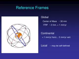
Reference Frames Global Center of Mass ~ 30 mm ITRF ~ 2 mm, < 1 mm/yr Continental < 1 mm/yr horiz., 2 mm/yr vert. Local -- may be self-defined
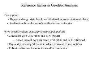
Reference frames in Geodetic Analyses Output from GAMIT • Loosely constrained solutions • Relative position well determined, “Absolute position” weakly defined • Need a procedure to expressed coordinates in a well defined reference frame Two aspects • Theoretical (e.g., rigid block, mantle-fixed, no-net-rotation of plates) • Realization through a set of coordinates and velocities - “finite constraints” : a priori sigmas on site coordinates - “generalized constraints” : minimize coordinate residuals while adjusting translation, rotation, and scale parameters Three considerations in data processing and analysis • Consistent with GPS orbits and EOP (NNR) -- not an issue if network small or if orbits and EOP estimated • Physically meaningful frame in which to visualize site motions • Robust realization for velocities and/or time series
Velocities of Anatolia and the Aegean in a Eurasian frameRealized by minimizing the velocities of 12 sites over the whole of Eurasia McClusky et al. [2000]
Velocities in an Anatolian frameBetter visualization of Anatolian and Aegean deformation McClusky et al. [2000]
Another example: southern Balkans Pan-Eurasian realization (as in last example) Note uniformity in error ellipses, dominated by frame uncertainty
Frame realization using 8 stations in central Macedonia Note smaller error ellipses within stabilization region and larger ellipses at edges
DefiningReference Frames in GLOBK • Three approaches to reference frame definition in GLOBK • Finite constraints ( in globk, same as GAMIT ) • Generalized constraints in 3-D ( in glorg ) • Generalized constraints for horizontal blocks (‘plate’ feature of glorg) • Reference frame for time series • More sensitive than velocity solution to changes in sites • Initially use same reference sites as velocity solution • Final time series should use (almost) all sites for stabilization
Frame definition with finite constraints Applied in globk (glorg not called) apr_file itrf05.apr apr_neu all 10 10 10 1 1 1 apr_neu algo .005 005 .010 .001 .001 .003 apr_neu pie1 .002 005 .010 .001 .001 .003 apr_neu drao .005 005 .010 .002 .002 .005 … • Most useful when only one or two reference sites • Disadvantage for large networks is that bad a priori coordinates or bad data from a reference site can distort the network
Frame definition with generalized constraints Applied in glorg: minimize residuals of reference sites while estimating translation, rotation, and/or scale (3 -7 parameters) apr_file itrf05.apr pos_org xtran ytran ztran xrot yrot zrot stab_site algo pie1 drao … cnd_hgtv 10 10 0.8 3. • All reference coordinates free to adjust (anomalies more apparent); outliers are iteratively removed by glorg • Network can translate and rotate but not distort • Works best with strong redundancy (number and [if rotation] geometry of coordinates exceeds number of parameters estimated) • Can downweight heights if suspect
Referencing to a horizontal block (‘plate’) Applied in glorg: first stabilize in the usual way with respect to a reference set of coordinates and velocities (e.g. ITRF-NNR), then define one or more ‘rigid’ blocks apr_file itrf05.apr pos_org xtran ytran ztran xrot yrot zrot stab_site algo pie1 nlib drao gold sni1 mkea chat cnd_hgtv 10 10 0.8 3. plate noam algo pie1 nlib plate pcfc sni1 mkea chat After stabilization, glorg will estimate a rotation vector (‘Euler pole’) for each plate with respect to the frame of the full stabilization set and print the relative poles between each set of plates Use sh_org2vel to extract the velocities of all sites with respect to each plate
Rules for Stabilization of Time Series • Small-extent network: translation-only in glorg, must constrain EOP in globk • Large-extent network: translation+rotation, must keep EOP loose in globk; if scale estimated in glorg, must estimate scale in globk • 1st pass for editing: - “Adequate” stab_site list of stations with accurate a priori coordinates and velocities and available most days - Keep in mind deficiencies in the list • Final pass for presentation / assessment / statistics - Robust stab_site list of all/most stations in network, with coordinates and velocities determined from the final velocity solution
Reference Frames in Time Series Spatial filtering of Time Series Example from southwest China Stabilization with respect to a pan-Eurasia station set Stabilization with respect to a SW-China station set: spatially correlated noise reduced; this time series best represents the uncertainties in the velocity solution
.. Same two solutions, East component Eurasia stabilization SW-China stabilization 1993: noise spatially correlated 1994: noise local
Stabilization Challenges for Time Series Network too wide to estimate translation-only (but reference sites too few or poorly distributed to estimate rotation robustly )
Stabilization Challenges for Time Series * Example of time series for which the available reference sites changes day-to-day but is robust (6 or more sites, well distributed, with translation and rotation estimated) Day 176 ALGO PIE1 DRAO WILL ALBH NANO rms 1.5 mm Day 177 ALGO NLIB CHUR PIE1 YELL DRAO WILL ALBH NANO rms 2.3 mm * ** ** ** ** ** * ** ^ ^ ^ ^
Stabilization Challenges for Time Series * Example of time series for which the available reference sites changes day-to-day and is not robust (only 3 sites on one day) Day 176 BRMU PIE1 WILL rms 0.4 mm Day 177 BRMU ALGO NLIB PIE1 YELL WILL rms 2.0 mm ** * * ** ** ^ ^ ^ ^ ^ ^ ^ ^
Include global h-files … or not ? Advantages • Access to a large number of sites for frame definition • Can (should) allow adjustment to orbits and EOP • Eases computational burden Disadvantages • Must use (mostly) the same models as the global processing • Orbits implied by the global data worse than IGSF • Some bad data may be included in global h-files (can remove) • Greater data storage burden
Regional versus Global stabilization If not using external h-files, use 8 or more well distributed sites reference sites If combining with MIT or SOPAC* global h-files, use 4-6 well-performing common sites (not necessarily with well-known coordinates), MIT hfiles availaibale at ftp://everest.mit.edu/pub/MIT_GLL/HYY* If SOPAC, use all “igs’ h-files to get orbits well-determined
Potential Reference Sites for South American Data ProcessingCriterions for IGS selectionsData availabilityA easy way to do it is to go tohttp://sopac.ucsd.edu/dataArchive/dataBrowser.htmlCoordinates quality in apr fileCheck time series and its length – SOPAC againGood coverage around your network make your own tests !
SITE DATA SPAN # DAYS # DATA (dec. yr) LOSS (%)----------------------------------------------------------------------ANTC : 001 2010 -> 365 2010 365 361 1.00 1.1 % AREQ : 001 2010 -> 365 2010 365 365 1.00 0.0 % BDOS : 001 2010 -> 365 2010 365 202 1.00 44.7 % BOGT : 001 2010 -> 365 2010 365 331 1.00 9.3 % BRAZ : 001 2010 -> 348 2010 365 331 1.00 4.9 % BRFT : 001 2010 -> 365 2010 365 270 1.00 26.0 % BRMU : 001 2010 -> 365 2010 365 353 1.00 3.3 % CFAG : 001 2010 -> 347 2010 365 347 1.00 0.0 % CHPI : 001 2010 -> 365 2010 365 359 1.00 1.6 % CONT : 001 2010 -> 365 2010 365 358 1.00 1.9 % CONZ : 001 2010 -> 365 2010 365 363 1.00 0.5 % COPO : 001 2010 -> 365 2010 365 362 1.00 0.8 % COYQ : 001 2010 -> 365 2010 365 225 1.00 38.4 % CRO1 : 001 2010 -> 365 2010 365 319 1.00 12.6 % FALK : 001 2010 -> 365 2010 365 342 1.00 6.3 % FORT : 001 2010 -> 365 2010 365 0 1.00 100.0 %GLPS : 001 2010 -> 362 2010 365 336 1.00 7.2 % GUAT : 001 2010 -> 280 2010 365 217 1.00 22.5 % INEG : 001 2010 -> 365 2010 365 365 1.00 0.0 % IQQE : 001 2010 -> 365 2010 365 347 1.00 4.9 %
Reference frame issues specific to South AmericaEarthquakes cause large co-seismic displacements, up to several metersand non linear post-seismic displacement, especially in the near field of the ruptured area
Impact of the MauleMw=8.8 2010 Earthquake on reference sites in South America
Reference frame issues specific to South America What to do for earthquakes? • Wait for an updated apr to be available • Add a line in the eq_rename file or define an earthquake • rename SANT SANT_4PS 2010 2 27 6 34 2100 1 1 0 0 • eq_def ma -72.963 -36.208, 500 35 2010 02 27 • SANT_4PS is not in the apr file and SANT will not be used in the stabilization • Globk can provide the co-seismic jump and new coordinates • However, SANT is likely to have a strong non-linear post-seismic behavior and could not be used for a while
Reference frame issues specific to South America Large seasonnal signals due to hydrological loading in the Amazonian basin May generates spurious signals in time series Courtesy J. P. Boy