Chapter 6 The Definite Integral
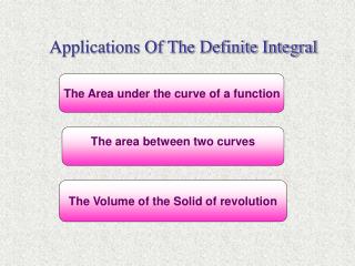
Chapter 6 The Definite Integral. Chapter Outline. Antidifferentiation Areas and Riemann Sums Definite Integrals and the Fundamental Theorem Areas in the xy -Plane Applications of the Definite Integral. § 6.1. Antidifferentiation. Section Outline. Antidifferentiation

Chapter 6 The Definite Integral
E N D
Presentation Transcript
Chapter Outline • Antidifferentiation • Areas and Riemann Sums • Definite Integrals and the Fundamental Theorem • Areas in the xy-Plane • Applications of the Definite Integral
§6.1 Antidifferentiation
Section Outline • Antidifferentiation • Finding Antiderivatives • Theorems of Antidifferentiation • The Indefinite Integral • Rules of Integration • Antiderivatives in Application
Antidifferentiation Goldstein/SCHNIEDER/LAY, CALCULUS AND ITS APPLICATIONS, 11e – Slide #5
Finding Antiderivatives EXAMPLE Find all antiderivatives of the given function. SOLUTION The derivative of x9 is exactly 9x8. Therefore, x9 is an antiderivative of 9x8. So is x9 + 5 and x9 -17.2. It turns out that all antiderivatives of f(x) are of the form x9 + C (where C is any constant) as we will see next. Goldstein/SCHNIEDER/LAY, CALCULUS AND ITS APPLICATIONS, 11e – Slide #6
Theorems of Antidifferentiation Goldstein/SCHNIEDER/LAY, CALCULUS AND ITS APPLICATIONS, 11e – Slide #7
The Indefinite Integral Goldstein/SCHNIEDER/LAY, CALCULUS AND ITS APPLICATIONS, 11e – Slide #8
Rules of Integration Goldstein/SCHNIEDER/LAY, CALCULUS AND ITS APPLICATIONS, 11e – Slide #9
Finding Antiderivatives EXAMPLE Determine the following. SOLUTION Using the rules of indefinite integrals, we have Goldstein/SCHNIEDER/LAY, CALCULUS AND ITS APPLICATIONS, 11e – Slide #10
Finding Antiderivatives EXAMPLE Find the function f(x) for which and f(1) = 3. SOLUTION The unknown function f(x) is an antiderivative of . One antiderivative is . Therefore, by Theorem I, Now, we want the function f(x) for which f(1) = 3. So, we must use that information in our antiderivative to determine C. This is done below. Goldstein/SCHNIEDER/LAY, CALCULUS AND ITS APPLICATIONS, 11e – Slide #11
Finding Antiderivatives CONTINUED So, 3 = 1 + C and therefore, C = 2. Therefore, our function is Goldstein/SCHNIEDER/LAY, CALCULUS AND ITS APPLICATIONS, 11e – Slide #12
Antiderivatives in Application EXAMPLE A rock is dropped from the top of a 400-foot cliff. Its velocity at time t seconds is v(t) = -32t feet per second. (a) Find s(t), the height of the rock above the ground at time t. (b) How long will the rock take to reach the ground? (c) What will be its velocity when it hits the ground? SOLUTION (a) We know that s΄(t) = v(t) = -32t and we also know that s(0) = 400. We can now use this information to find an antiderivative of v(t) for which s(0) = 400. The antiderivative of v(t) is To determine C, Therefore, C = 400. So, our antiderivative is s(t) = -16t2 + 400. Goldstein/SCHNIEDER/LAY, CALCULUS AND ITS APPLICATIONS, 11e – Slide #13
Antiderivatives in Application CONTINUED (b) To determine how long it will take for the rock to reach the ground, we simply need to find the value of t for which the position of the rock is at height 0. In other words, we will find t for when s(t) = 0. s(t) = -16t2 + 400 This is the function s(t). 0 = -16t2 + 400 Replace s(t) with 0. -400 = -16t2 Subtract. 25 = t2 Divide. 5 = t Take the positive square root since t≥ 0. So, it will take 5 seconds for the rock to reach the ground. Goldstein/SCHNIEDER/LAY, CALCULUS AND ITS APPLICATIONS, 11e – Slide #14
Antiderivatives in Application CONTINUED (c) To determine the velocity of the rock when it hits the ground, we will need to evaluate v(5). v(t) = -32t This is the function v(t). Replace t with 5 and solve. v(5) = -32(5) = -160 So, the velocity of the rock, as it hits the ground, is 160 feet per second in the downward direction (because of the minus sign). Goldstein/SCHNIEDER/LAY, CALCULUS AND ITS APPLICATIONS, 11e – Slide #15
§6.2 Areas and Riemann Sums
Section Outline • Area Under a Graph • Riemann Sums to Approximate Areas (Midpoints) • Riemann Sums to Approximate Areas (Left Endpoints) • Applications of Approximating Areas
Area Under a Graph Goldstein/SCHNIEDER/LAY, CALCULUS AND ITS APPLICATIONS, 11e – Slide #18
Area Under a Graph In this section we will learn to estimate the area under the graph of f(x) from x = a to x = b by dividing up the interval into partitions (or subintervals), each one having width where n = the number of partitions that will be constructed. In the example below, n = 4. A Riemann Sum is the sum of the areas of the rectangles generated above. Goldstein/SCHNIEDER/LAY, CALCULUS AND ITS APPLICATIONS, 11e – Slide #19
Riemann Sums to Approximate Areas EXAMPLE Use a Riemann sum to approximate the area under the graph f(x) on the given interval using midpoints of the subintervals SOLUTION The partition of -2 ≤ x ≤ 2 with n = 4 is shown below. The length of each subinterval is x1 x2 x3 x4 -2 2 Goldstein/SCHNIEDER/LAY, CALCULUS AND ITS APPLICATIONS, 11e – Slide #20
Riemann Sums to Approximate Areas CONTINUED Observe the first midpoint is units from the left endpoint, and the midpoints themselves are units apart. The first midpoint is x1 = -2 + = -2 + .5 = -1.5. Subsequent midpoints are found by successively adding midpoints: -1.5, -0.5, 0.5, 1.5 The corresponding estimate for the area under the graph of f(x) is So, we estimate the area to be 5 (square units). Goldstein/SCHNIEDER/LAY, CALCULUS AND ITS APPLICATIONS, 11e – Slide #21
Approximating Area With Midpoints of Intervals CONTINUED Goldstein/SCHNIEDER/LAY, CALCULUS AND ITS APPLICATIONS, 11e – Slide #22
Riemann Sums to Approximate Areas EXAMPLE Use a Riemann sum to approximate the area under the graph f(x) on the given interval using left endpoints of the subintervals SOLUTION The partition of 1 ≤ x ≤ 3 with n = 5 is shown below. The length of each subinterval is 1 1.4 1.8 2.2 2.6 3 x1 x2 x3 x4 x5 Goldstein/SCHNIEDER/LAY, CALCULUS AND ITS APPLICATIONS, 11e – Slide #23
Riemann Sums to Approximate Areas CONTINUED The corresponding Riemann sum is So, we estimate the area to be 15.12 (square units). Goldstein/SCHNIEDER/LAY, CALCULUS AND ITS APPLICATIONS, 11e – Slide #24
Approximating Area Using Left Endpoints CONTINUED Goldstein/SCHNIEDER/LAY, CALCULUS AND ITS APPLICATIONS, 11e – Slide #25
Applications of Approximating Areas EXAMPLE The velocity of a car (in feet per second) is recorded from the speedometer every 10 seconds, beginning 5 seconds after the car starts to move. See Table 2. Use a Riemann sum to estimate the distance the car travels during the first 60 seconds. (Note: Each velocity is given at the middle of a 10-second interval. The first interval extends from 0 to 10, and so on.) SOLUTION Since measurements of the car’s velocity were taken every ten seconds, we will use . Now, upon seeing the graph of the car’s velocity, we can construct a Riemann sum to estimate how far the car traveled. Goldstein/SCHNIEDER/LAY, CALCULUS AND ITS APPLICATIONS, 11e – Slide #26
Applications of Approximating Areas CONTINUED Goldstein/SCHNIEDER/LAY, CALCULUS AND ITS APPLICATIONS, 11e – Slide #27
Applications of Approximating Areas CONTINUED Therefore, we estimate that the distance the car traveled is 2800 feet. Goldstein/SCHNIEDER/LAY, CALCULUS AND ITS APPLICATIONS, 11e – Slide #28
§6.3 Definite Integrals and the Fundamental Theorem
Section Outline • The Definite Integral • Calculating Definite Integrals • The Fundamental Theorem of Calculus • Area Under a Curve as an Antiderivative
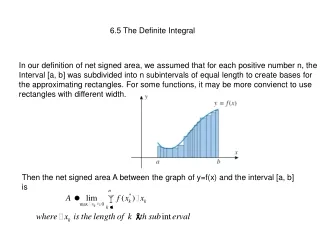
The Definite Integral Δx = (b – a)/n, x1, x2, …., xn are selected points from a partition [a, b]. Goldstein/SCHNIEDER/LAY, CALCULUS AND ITS APPLICATIONS, 11e – Slide #31
Calculating Definite Integrals EXAMPLE Calculate the following integral. SOLUTION The figure shows the graph of the function f(x) = x + 0.5. Since f(x) is nonnegative for 0 ≤ x ≤ 1, the definite integral of f(x) equals the area of the shaded region in the figure below. 1 1 0.5 Goldstein/SCHNIEDER/LAY, CALCULUS AND ITS APPLICATIONS, 11e – Slide #32
Calculating Definite Integrals CONTINUED The region consists of a rectangle and a triangle. By geometry, Thus the area under the graph is 0.5 + 0.5 = 1, and hence Goldstein/SCHNIEDER/LAY, CALCULUS AND ITS APPLICATIONS, 11e – Slide #33
The Definite Integral Goldstein/SCHNIEDER/LAY, CALCULUS AND ITS APPLICATIONS, 11e – Slide #34
Calculating Definite Integrals EXAMPLE Calculate the following integral. SOLUTION The figure shows the graph of the function f(x) = x on the interval -1 ≤ x ≤ 1. The area of the triangle above the x-axis is 0.5 and the area of the triangle below the x-axis is 0.5. Therefore, from geometry we find that Goldstein/SCHNIEDER/LAY, CALCULUS AND ITS APPLICATIONS, 11e – Slide #35
Calculating Definite Integrals CONTINUED Goldstein/SCHNIEDER/LAY, CALCULUS AND ITS APPLICATIONS, 11e – Slide #36
The Fundamental Theorem of Calculus Goldstein/SCHNIEDER/LAY, CALCULUS AND ITS APPLICATIONS, 11e – Slide #37
The Fundamental Theorem of Calculus EXAMPLE Use the Fundamental Theorem of Calculus to calculate the following integral. SOLUTION An antiderivative of 3x1/3 – 1 – e0.5x is . Therefore, by the fundamental theorem, Goldstein/SCHNIEDER/LAY, CALCULUS AND ITS APPLICATIONS, 11e – Slide #38
The Fundamental Theorem of Calculus EXAMPLE (Heat Diffusion) Some food is placed in a freezer. After t hours the temperature of the food is dropping at the rate of r(t) degrees Fahrenheit per hour, where (a) Compute the area under the graph of y = r(t) over the interval 0 ≤ t ≤ 2. (b) What does the area in part (a) represent? SOLUTION (a) To compute the area under the graph of y = r(t) over the interval 0 ≤ t ≤ 2, we evaluate the following. Goldstein/SCHNIEDER/LAY, CALCULUS AND ITS APPLICATIONS, 11e – Slide #39
The Fundamental Theorem of Calculus CONTINUED (b) Since the area under a graph can represent the amount of change in a quantity, the area in part (a) represents the amount of change in the temperature between hour t = 0 and hour t = 2. That change is 24.533 degrees Fahrenheit. Goldstein/SCHNIEDER/LAY, CALCULUS AND ITS APPLICATIONS, 11e – Slide #40
Area Under a Curve as an Antiderivative Goldstein/SCHNIEDER/LAY, CALCULUS AND ITS APPLICATIONS, 11e – Slide #41
§6.4 Areas in the xy-Plane
Section Outline • Properties of Definite Integrals • Area Between Two Curves • Finding the Area Between Two Curves
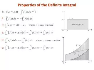
Properties of Definite Integrals Goldstein/SCHNIEDER/LAY, CALCULUS AND ITS APPLICATIONS, 11e – Slide #44
Area Between Two Curves Goldstein/SCHNIEDER/LAY, CALCULUS AND ITS APPLICATIONS, 11e – Slide #45
Finding the Area Between Two Curves EXAMPLE Find the area of the region between y = x2 – 3x and the x-axis (y = 0) from x = 0 to x = 4. SOLUTION Upon sketching the graphs we can see that the two graphs cross; and by setting x2 – 3x = 0, we find that they cross when x = 0 and when x = 3. Thus one graph does not always lie above the other from x = 0 to x = 4, so that we cannot directly apply our rule for finding the area between two curves. However, the difficulty is easily surmounted if we break the region into two parts, namely the area from x = 0 to x = 3 and the area from x = 3 to x = 4. For from x = 0 to x = 3, y = 0 is on top; and from x = 3 to x = 4, y = x2 – 3x is on top. Consequently, Goldstein/SCHNIEDER/LAY, CALCULUS AND ITS APPLICATIONS, 11e – Slide #46
Finding the Area Between Two Curves CONTINUED Thus the total area is 4.5 + 1.833 = 6.333. Goldstein/SCHNIEDER/LAY, CALCULUS AND ITS APPLICATIONS, 11e – Slide #47
Finding the Area Between Two Curves CONTINUED y = x2 – 3x y = 0 Goldstein/SCHNIEDER/LAY, CALCULUS AND ITS APPLICATIONS, 11e – Slide #48
Finding the Area Between Two Curves EXAMPLE Write down a definite integral or sum of definite integrals that gives the area of the shaded portion of the figure. SOLUTION Since the two shaded regions are (1) disjoint and (2) have different functions on top, we will need a separate integral for each. Therefore Goldstein/SCHNIEDER/LAY, CALCULUS AND ITS APPLICATIONS, 11e – Slide #49
Finding the Area Between Two Curves CONTINUED Therefore, to represent all the shaded regions, we have Goldstein/SCHNIEDER/LAY, CALCULUS AND ITS APPLICATIONS, 11e – Slide #50