Download
1 / 64
640 likes | 763 Vues
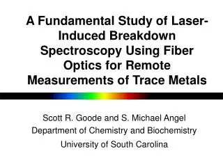
A Fundamental Study of Laser-Induced Breakdown Spectroscopy Using Fiber Optics for Remote Measurements of Trace Metals. Scott R. Goode and S. Michael Angel Department of Chemistry and Biochemistry University of South Carolina. LIBS for Elemental Analysis. Approach Fiber optic technology

E N D
A Fundamental Study of Laser-Induced Breakdown Spectroscopy Using Fiber Optics for Remote Measurements of Trace Metals Scott R. Goode and S. Michael Angel Department of Chemistry and Biochemistry University of South Carolina
LIBS for Elemental Analysis • Approach • Fiber optic technology • Wavelength resolution • Time resolution • Accomplishments • Two operating instruments • Examining surface morphology • Studying matrix effects • Future • Solutions and slurries
Laser-Induced Breakdown Spectroscopy • Use laser to vaporize sample • Laser electric field high enough to cause breakdown • Monitor emission • Fiber optics afford capability for remote analysis
Limiting Factor • Discriminating analyte atomic emission from continuum background emission limits the analysis • Time • Wavelength
1064 nm mirror Pulsed Laser focusing lens collection lens intensified detector Spectrograph plasma Timing Control Time-Resolved LIBS Apparatus
Laser trigger Fiber-Optic LIBS System Configuration Pulsed laser Lens Delay generator Detector Lens Controller Fiber-optic LIBS probe Spectrograph Computer
Fiber-Optic LIBS Probe Design f/2 Lens Plasma Collection Fiber Excitation Fiber Focusing lens Sample
Lead in Paint Using Fiber-Optic LIBS Probe 1400 1200 Pb Ti Ti Ti 1000 Solder 800 Intensity Leaded Paint 600 400 Unleaded Paint 200 0 398.0 400.0 402.0 404.0 406.0 Wavelength (nm)
Leaded Paint Calibration Using Fiber-Optic Probe 200 - 4 mJ/pulse, 2 Hz, 532 nm laser, avg. 5 replicate spectra 150 Intensity 100 50 L.O.D.= 0.014% Pb (wt/wt) Dry Basis 0 0.00 0.02 0.04 0.06 0.08 0.10 Concentration of Lead (% w/w, Dry Basis)
Fiber-Optic Transmission 120 110 1 mm silica-clad 1 mm hard-clad 800 m hard-clad 600 m hard-clad 100 90 80 70 Power Out of fiber (mJ) 60 50 fiber breakdown 40 30 20 10 0 10 20 30 40 50 60 70 80 90 100 110 120 130 140 150 Power into Fiber (mJ)
spectral excit. 10x Ar+ imaging ex. w/GRIN pellicle excitation fiber f/8 LIBS/Raman collection fiber Nd:YAG imaging fiber He:Ne 6xmacro lens imaging fiber 10x b&w CCD frame grabber f/7 lens ICCD monitor probe pulser controller spectrograph
Video camera Collection fiber (filtered for Raman) LIBS excitation fiber (1064 nm) (632 nm pointer) Filtered Raman excitation fiber (514.5 nm) Imaging fiber GRIN lens Region of interest Imaged region Sample
5 mm Fe Ca 35x103 a b Fe Fe 25 Fe Intensity Fe 15 Fe 5 404 408 412 416 420 Wavelength (nm) Region of Interest 16 x103 c d Ca Sr 14 Sr Intensity 10 6 2 404 408 412 416 420 Wavelength (nm)
Raman spectrum of TiO2 b 200x103 Darkfield image of TiO2 and Sr(NO3)2 on soil 150 Intensity 100 a 50 0 200 400 600 800 1000 Wavenumber (cm-1) Raman spectrum of Sr(NO3)2 c 200x103 150 Intensity 100 50 800 1000 1200 1400 1600 Wavenumber (cm-1)
Raman Images TiO2 @190 cm-1 Darkfield image of TiO2 and Sr(NO3)2 on soil b a Sr(NO3 ) 2 @1055cm-1 c
Graph 7 (top of plasma) Top Graph 6 Bottom Plasma Temperature Profile Regions 2500 7 7 0 366 368 370 372 374 376 378 380 382 384 2500 6 6 0 366 368 370 372 374 376 378 380 382 384 Graph 5 2500 5 5 0 366 368 370 372 374 376 378 380 382 384 Graph 4 2500 4 4 0 Observed plasma region 366 368 370 372 374 376 378 380 382 384 Graph 3 2500 3 3 0 366 368 370 372 374 376 378 380 382 384 Graph 2 2500 2 2 0 366 368 370 372 374 376 378 380 382 384 Graph 1 (bottom of plasma) 2500 1 1 0 366 368 370 372 374 376 378 380 382 384 6000 7000 Plasma temperature (K)
LIBS Imaging Spectrometer 1064 nm mirror laser beam stop ICCD AOTF lens 1064 nm mirror sample collimating lens plasma RF generator
mm 2 .64 Background Subtracted Lead Emission Repetition Rate: 2 Hz, 2000 Shots, 2.5 s Delay 722.8 nm Lead Emission + Continuum 715.2 nm Continuum Background Background Subtracted
Continuum background Temporal Dependence of Lead Emission Background subtracted Pb emission at 722.8 nm 2.5 mm 2.5 mm 50 ns 675 ns 1. 3 ms 1. 9 ms 2. 5 ms
960 shots 2400 shots 100 shots 1.42 mm mm 0.63 Lead Crater Depth and Plasma Height 0.38 mm 0.50 mm 0.38 mm mm 2.75
Plasma Height vs. Number of Laser Shots Rep Rate: 2 Hz 2.5 s delay 2500 1.0 s delay 2000 Plasma Height (microns) 1500 1000 500 1000 1500 2000 Number of Laser Shots
Using High Wavelength Resolution If the major source of noise is the continuum background • Eliminate the background by time resolution • Use wavelength resolution to distinguish the atomic lines from the continuum background
Matrix effects • Use binary alloy (brass samples) • Examine signals from zinc (volatile) and copper (nonvolatile) • Vary laser power • Vary focal depth
Studying selective volatilization • Measure zinc and copper emission from brass standards • Perform measurements while varying laser power (Q-switch delay) • See if ratio is independent of power and proportional to concentration
Effect of focus • Measure Zn-to-Cu emission ratio • As a function of composition • As a function of focal point • Negative: focal point below surface • Zero: at surface • Positive: above surface
Conclusions • LIBS is more complex than originally thought. • Much of the data are consistent with a low-power heating mechanism and a high power dielectric vaporization mechanism. • Can design experiments to decouple excitation and vaporization.
Segregate excitation effects from vaporization effects • Brass samples, known composition • Laser ablation into solution • Dissolution • Chemical analysis by ICP-MS • Determine if materials vaporized in proportion to concentration • Determine factors that affect selective and nonselective vaporization
Spectrometer • High Spectral Resolution (7500) • High Time Resolution (5 ns) • Delivery?
Alternative Excitation • Use laser system to vaporize solid sample. • Direct vapor into microwave-excited plasma. • Use emission from microwave plasma for chemical analysis.
Colinear Dual-Pulse LIBS Configuration Pulser ICCD Controller Pulsed Nd:YAG Optical Fiber Spectrograph lens Timing Control 1064nm mirror lens Pulsed Nd:YAG plasma sample
1064 nm Laser 1 (100 mJ) Laser 2 (180 mJ) Colinear Dual-Pulse LIBS Enhancement for Copper 3 0 s between lasers 25x10 1 s between lasers 20 15 Intensity (arb units) 10 5 500 505 510 515 520 525 530 Wavelength (nm)
Time Between Lasers (s) Optimum Delay Between Lasers for Copper Enhancement 16 Colinear Dual-Pulse LIBS 14 12 Laser 1 = 100 mJ Laser 2 = 180 mJ Signal-to-Bkg 10 8 6 4 2 0 100 200 300 400 500
Copper Craters from Colinear Dual-Pulse LIBS 0 s T 1 s T 20 s T 0.38 mm 0.38 mm 0.38 mm Cu S/B 3 Cu S/B 14 Cu S/B 15
Optimum Timing Between Lasers for Lead Enhancement Colinear Dual-Pulse LIBS 4.0 3.5 Pb SBR 3.0 2.5 100 0 20 40 60 80 Time Between Lasers ( s) T
Comparison of Lead Craters (colinear geometry) Zero s T One s T 0.60 mm 0.60 mm Pb S/B 6 Pb S/B 2.5
Orthogonal Dual-Pulse LIBS Nd:YAG Pulser ICCD Controller Timing Control Spectrograph plasma Nd:YAG