Download

1 / 86
860 likes | 1.01k Vues
CSE 332 Data Abstractions: Priority Queues, Heaps, and a Small Town Barber. Kate Deibel Summer 2012. Announcements. David's Super Awesome Office Hours Mondays 2:30-3:30 CSE 220 Wednesdays 2:30-3:30 CSE 220 Sundays 1:30-3:30 Allen Library Research Commons Or by appointment

E N D
CSE 332 Data Abstractions:Priority Queues, Heaps, and a Small Town Barber Kate Deibel Summer 2012 CSE 332 Data Abstractions, Summer 2012
Announcements David's Super Awesome Office Hours • Mondays 2:30-3:30 CSE 220 • Wednesdays 2:30-3:30 CSE 220 • Sundays 1:30-3:30 Allen Library Research Commons • Or by appointment Kate's Fairly Generic But Good Quality Office Hours • Tuesdays, 2:30-4:30 CSE 210 • Whenever my office door is open • Or by appointment CSE 332 Data Abstractions, Summer 2012
Announcements • Remember to use cse332-staff@cs • Or at least e-mail both me and David • Better chance of a speedy reply • Kate is not available on Thursdays • I've decided to make Thursdays my focus on everything but Teaching days • I will not answer e-mails received on Thursdays until Friday CSE 332 Data Abstractions, Summer 2012
Today • Amortized Analysis Redux • Review of Big-Oh times for Array, Linked-List and Tree Operations • Priority Queue ADT • Heap Data Structure CSE 332 Data Abstractions, Summer 2012
Thinking beyond one isolated operation Amortized Analysis CSE 332 Data Abstractions, Summer 2012
Amortized Analysis • What happens when we have a costly operation that only occurs some of the time? • Example: My array is too small. Let's enlarge it. Option 1: Increase array size by 5 Copy old array into new one Option 2: Double the array size Copy old array into new one We will now explore amortized analysis! CSE 332 Data Abstractions, Summer 2012
Stretchy Array (version 1) StretchyArray: maxSize: positive integer (starts at 0) array: an array of size maxSize count: number of elements in array put(x): add x to the end of the array if maxSize == count make new array of size (maxSize + 5) copy old array contents to new array maxSize = maxSize + 5 array[count] = x count = count + 1 CSE 332 Data Abstractions, Summer 2012
Stretchy Array (version 2) StretchyArray: maxSize: positive integer (starts at 0) array: an array of size maxSize count: number of elements in array put(x): add x to the end of the array if maxSize == count make new array of size (maxSize * 2) copy old array contents to new array maxSize = maxSize * 2 array[count] = x count = count + 1 CSE 332 Data Abstractions, Summer 2012
Performance Cost of put(x) In both stretchy array implementations, put(x)is defined as essentially:if maxSize == count make new array of bigger size copy old array contents to new array update maxSize array[count] = x count = count + 1 What f(n) is put(x) in O( f(n) )? CSE 332 Data Abstractions, Summer 2012
Performance Cost of put(x) In both stretchy array implementations, put(x)is defined as essentially:if maxSize == count O(1) make new array of bigger size O(1) copy old array contents to new array O(n) update maxSizeO(1) array[count] = x O(1) count = count + 1 O(1) In the worst-case, put(x) is O(n) where n is the current size of the array!! CSE 332 Data Abstractions, Summer 2012
But… • We do not have to enlarge the array each time we call put(x) • What will be the average performance if we put n items into the array? O(?) • Calculating the average cost for multiple calls is known as amortized analysis CSE 332 Data Abstractions, Summer 2012
Amortized Analysis of StretchyArray Version 1 CSE 332 Data Abstractions, Summer 2012
Amortized Analysis of StretchyArray Version 1 Every five steps, we have to do a multiple of five more work CSE 332 Data Abstractions, Summer 2012
Amortized Analysis of StretchyArray Version 1 Assume the number of puts is n=5k • We will make n calls to array[count]=x • We will stretch the array k times and will cost: 0 + 5 + 10 + ⋯+ 5(k-1) Total cost is then: n + (0 + 5 + 10 + ⋯+ 5(k-1)) = n + 5(1 + 2 + ⋯+(k-1)) = n + 5(k-1)(k-1+1)/2 = n + 5k(k-1)/2 ≈ n + n2/10 Amortized cost for put(x) is CSE 332 Data Abstractions, Summer 2012
Amortized Analysis of StretchyArray Version 2 CSE 332 Data Abstractions, Summer 2012
Amortized Analysis of StretchyArray Version 2 Enlarge steps happen basically when i is a power of 2 CSE 332 Data Abstractions, Summer 2012
Amortized Analysis of StretchyArray Version 2 Assume the number of puts is n=2k • We will make n calls to array[count]=x • We will stretch the array k times and will cost: ≈1 + 2 + 4 + ⋯+ 2k-1 Total cost is then: ≈ n + (1 + 2 + 4 + ⋯+ 2k-1) ≈ n + 2k – 1 ≈ 2n - 1 Amortized cost for put(x) is CSE 332 Data Abstractions, Summer 2012
The Lesson With amortized analysis, we know that over the long run (on average): • If we stretch an array by a constant amount, each put(x) call is O(n) time • If we double the size of the array each time, each put(x) call is O(1) time In general, paying a high-cost infrequently can pay off over the long run. CSE 332 Data Abstractions, Summer 2012
What about wasted space? Two options: • We can adjust our growth factor • As long as we multiply the size of the array by a factor >1, amortized analysis holds • We can also shrink the array: • A good rule of thumb is to halve the array when it is only 25% full • Same amortized cost CSE 332 Data Abstractions, Summer 2012
Memorize these. They appear all the time. Array, List, and Tree performance CSE 332 Data Abstractions, Summer 2012
Very Common Interactions When we are working with data, there are three very common operations: • Insert(x): insert x into structure • Find(x): determine if x is in structure • Remove(i): remove item as position i • Delete(x): find and delete x from structure Note that when we usually delete, we • First find the element to remove • Then we remove it Overall time is O(Find + Remove) CSE 332 Data Abstractions, Summer 2012
Arrays and Linked Lists • Most common data structures • Several variants • Unsorted Array • Unsorted Circular Array • Unsorted Linked List • Sorted Array • Sorted Circular Array • Sorted Linked List • We will ignore whether the list is singly or doubly-linked • Usually only leads to a constant factor change in overall performance CSE 332 Data Abstractions, Summer 2012
Binary Search Tree (BST) • Another common data structure • Each node has at most two children • Left child's value is less than its parent • Right child's value is greater than parent • Structure depends on order elements were inserted into tree • Best performance occursif the tree is balanced • General properties • Min is leftmost node • Max is rightmost node 50 20 80 14 34 78 17 79 CSE 332 Data Abstractions, Summer 2012
Worst-Case Run-Times CSE 332 Data Abstractions, Summer 2012
Worst-Case Run-Times CSE 332 Data Abstractions, Summer 2012
Remove in an Unsorted Array • Let's say we want to remove the item at positioniin the array • All that we do is move the last item in the array to position i last item ⋯ ⋯ i last item ⋯ ⋯ i CSE 332 Data Abstractions, Summer 2012
Remove in a Binary Search Tree Replace node based on following logic • If no children, just remove it • If only one child, replace node with child • If two children, replace node with the smallest data for the right subtree • See Weiss 4.3.4 for implementation details CSE 332 Data Abstractions, Summer 2012
Balancing a Tree How do you guarantee that a BST will always be balanced? • Non-trivial task • We will discuss several implementations next Monday CSE 332 Data Abstractions, Summer 2012
The immediate priority is to discuss heaps. Priority Queues CSE 332 Data Abstractions, Summer 2012
Scenario What is the difference between waiting for service at a pharmacy versus an ER? Pharmacies usually follow the ruleFirst Come, First Served Emergency Rooms assign priorities based on each individual's need Queue PriorityQueue CSE 332 Data Abstractions, Summer 2012
New ADT: Priority Queue Each item has a “priority” • The next/best item has the lowest priority • So “priority 1” should come before “priority 4” • Could also do maximum priority if so desired Operations: • insert • deleteMin deleteMin returns/deletes item with lowest priority • Any ties are resolved arbitrarily • Fancier PQueues may use a FIFO approach for ties 6 2 15 23 12 18 45 3 7 insert deleteMin CSE 332 Data Abstractions, Summer 2012
Priority Queue Example insertawith priority 5 insertbwith priority 3 insertcwith priority 4 w= deleteMin x= deleteMin insertd with priority 2 inserte with priority 6 y= deleteMin z= deleteMin after execution: w= b x= c y= d z= a To simplify our examples, we will just use the priority values from now on CSE 332 Data Abstractions, Summer 2012
Applications of Priority Queues PQueues are a major and common ADT • Forward network packets by urgency • Execute work tasks in order of priority • “critical” before “interactive” before “compute-intensive” tasks • allocating idle tasks in cloud environments • A fairly efficient sorting algorithm • Insert all items into the PQueue • Keep calling deleteMin until empty CSE 332 Data Abstractions, Summer 2012
Advanced PQueue Applications • “Greedy” algorithms • Efficiently track what is “best” to try next • Discrete event simulation (e.g., virtual worlds, system simulation) • Every event e happens at some time t and generates new events e1, …, en at times t+t1, …, t+tn • Naïve approach: • Advance “clock” by 1, check for events at that time • Better approach: • Place events in a priority queue (priority = time) • Repeatedly: deleteMin and then insert new events • Effectively “set clock ahead to next event” CSE 332 Data Abstractions, Summer 2012
From ADT to Data Structure • How will we implement our PQueue? • We need to add one more analysis to the above: finding the min value CSE 332 Data Abstractions, Summer 2012
Finding the Minimum Value CSE 332 Data Abstractions, Summer 2012
Finding the Minimum Value CSE 332 Data Abstractions, Summer 2012
Best Choice for the PQueue? CSE 332 Data Abstractions, Summer 2012
None are that great We generally have to pay linear time for either insert or deleteMin • Made worse by the fact that:# inserts ≈ # deleteMins Balanced trees seem to be the best solution with O(log n) time for both • But balanced trees are complex structures • Do we really need all of that complexity? CSE 332 Data Abstractions, Summer 2012
Our Data Structure: The Heap Key idea: Only pay for functionality needed • Do better than scanning unsorted items • But do not need to maintain a full sort The Heap: • O(log n) insert and O(log n) deleteMin • If items arrive in random order, then the average-case of insert is O(1) • Very good constant factors CSE 332 Data Abstractions, Summer 2012
Reviewing Some Tree Terminology root(T): leaves(T): children(B): parent(H): siblings(E): ancestors(F): descendents(G): subtree(G): A D-F, I, J-N D, E, F G D, F B, A H, I, J-N G and itschildren Tree T A B C D E F G H I J K L M N CSE 332 Data Abstractions, Summer 2012
Some More Tree Terminology # edges depth(B): height(G): height(T): degree(B): branching factor(T): 1 2 4 3 0-5 Tree T A # edges on path from root to self B C # edges on longest path from node to leaf D E F G H I # children of a node MAX # children of a node for a BST this is?? J K L M N CSE 332 Data Abstractions, Summer 2012
Types of Trees • Binary tree: Every node has ≤2 children • n-ary tree: Every node as ≤n children • Perfect tree: Every row is completely full • Complete tree: All rows except the bottom are completely full, and it is filled from left to right Perfect Tree Complete Tree CSE 332 Data Abstractions, Summer 2012
Some Basic Tree Properties Nodes in a perfect binary tree of height h? 2h+1-1 Leaves in a perfect binary tree of height h? 2h Height of a perfect binary tree with n nodes? ⌊log2 n⌋ Height of a complete binary tree with n nodes? ⌊log2 n⌋ CSE 332 Data Abstractions, Summer 2012
Properties of a Binary Min-Heap More commonly known as a binary heap or simply a heap • Structure Property: A complete [binary] tree • Heap Property: The priority of every non-root node is greater than the priority of its parent How is this different from a binary search tree? CSE 332 Data Abstractions, Summer 2012
Properties of a Binary Min-Heap More commonly known as a binary heap or simply a heap • Structure Property: A complete [binary] tree • Heap Property: The priority of every non-root node is greater than the priority of its parent 30 10 20 80 20 80 13 25 40 60 85 99 A Heap Not a Heap 50 700 CSE 332 Data Abstractions, Summer 2012
Properties of a Binary Min-Heap • Where is the minimum priority item? At the root • What is the height of a heap with n items? ⌊log2 n⌋ 10 20 80 40 60 85 99 A Heap 50 700 CSE 332 Data Abstractions, Summer 2012
Basics of Heap Operations findMin: • return root.data deleteMin: • Move last node up to root • Violates heap property, so Percolate Down to restore insert: • Add node after last position • Violate heap property, so Percolate Up to restore 10 • The general idea: • Preserve the complete tree structure property • This likely breaks the heap property • So percolate to restore the heap property 20 80 40 60 85 99 50 700 CSE 332 Data Abstractions, Summer 2012
DeleteMin Implementation 1. Delete value at root node (and store it for later return) • There is now a "hole" at the root. We must "fill" the hole with another value, must have a tree with one less node, and it must still be a complete tree • The "last" node is the is obvious choice, but now the heap property is violated • We percolate down to fix the heap While greater than either child Swap with smaller child 4 3 7 5 8 9 11 9 6 10 10 4 3 7 5 8 9 11 9 6 10 CSE 332 Data Abstractions, Summer 2012
Percolate Down While greater than either child Swap with smaller child ? 10 3 3 ? 4 3 4 4 8 10 ? 7 5 8 9 7 5 8 9 7 5 9 10 11 9 6 11 9 6 11 9 6 What is the runtime? O(log n) Why does this work? Both children are heaps CSE 332 Data Abstractions, Summer 2012