Download

1 / 69
710 likes | 1.03k Vues
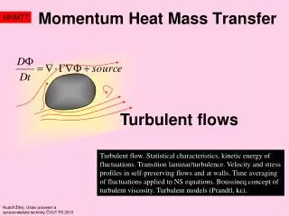
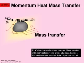
Momentum Heat Mass Transfer. MHMT3. Kinematics and dynamics. Constitutive equations. Kinematics of deformation , stresses, invariants and r heological constitutive equations . Fluids, solids and viscoelastic materials . Rudolf Žitný, Ústav procesní a zpracovatelské techniky ČVUT FS 2010.

E N D
Momentum Heat Mass Transfer MHMT3 Kinematics and dynamics. Constitutive equations Kinematics of deformation, stresses, invariants and rheological constitutive equations. Fluids, solids and viscoelastic materials. Rudolf Žitný, Ústav procesní a zpracovatelské techniky ČVUT FS 2010
Constitutive equations MHMT3 Material (fluid, solid) reacts by inner forces only if the body is deformed or in nonhomogeneous flows. deformation Stresses in elastic solids depend only upon the stretching of a short material „fiber“. Stretching of fibers depends upon the initial fiber orientation. Stresses are independent of the rate of stretching and of the rigid body motion (translation and rotation). Deformation is reversible, after removal of external forces, original configuration is restored. l0 l0 Material with memory Stresses in viscous fluids depend only upon the rate of changes of distance between neighboring molecules. The distance changes are caused by nonuniform velocity field (by nonzero velocity gradient). Stresses are again independent of the rigid body motion (translation and rotation). Process is irreversible and molecules have no memory of an initial configuration (stresses are caused by relative motion of instantaneous neighbors). Material without memory Many materials are something between – viscoelastic fluids have partial memory (fading memory). Example: polymers, food products…
Constitutive equations MHMT3 Kinematic variables in solids and fluids Reference and deformed configuration is distinguished. Motion is described by displacement of material particles. reference configuration displacement l0 l0 stretch Solids Only the current configuration is considered (changes of configuration during infinitely short time interval dt). Motion is described by velocities of material particles. velocity time t+dt time t Fluids Velocity is the time derivative of displacement
Constitutive equations FLUID MHMT3 Motion of viscous fluid is a fully irreversible process, mechanical energy is converted to heat. Fluid has no memory to previous spatial configuration of fluid particle, there is no recoil after unloading external stress. Newton’s law: Macke
Fluids: Kinematics of flow MHMT3 In case of fluids without a long time memory the role of displacements (differences between the current and the reference position of material particles) is taken over by the fluid velocities at near points. Viscous stresses are response to changing distances, for example between the near points A,B during the time dt. B’ Gradient of velocity A’ Arbitrary tensor can be decomposed to the sum of symmetric and antisymmetric part B A Spin (antisymmetric) Rate of deformation
Fluids: Kinematics of flow B’ A’ B A MHMT3 Result can be expressed as Helmholtz kinematic theorem, stating that any motion of fluid can be decomposed to translation + rotation + deformation Vorticity tensor Rate of deformation tensor Viscous stresses are not affected by translation nor by rotation (tensor of spin, vorticity), because these modes of motion preserve distance between the nearest fluid particles.
Fluids: stresses MHMT3 • Tensor of total stresses can be decomposed to pressure and viscous stresses • Hydrostatic pressure (isotropic, independent of relative motion of fluid particles). For pure fluids the pressure can be derived from thermodynamics relationships, • e.g. where u is internal energy and s – entropy. • Viscous stresses are fully described by a symmetric tensor independent of the rigid body motion. Viscous stress is in fact the momentum flux due to molecular diffusion.
Fluids: Constitutive equation MHMT3 Constitutive equations represent a relationship between Kinematics(characterised by the rate of deformation for fluids) Viscous stress(dynamic response to deformation) The simplest constitutive equation for purely viscous (Newtonian) fluids is linear relationship between the tensor of viscous stresses and the tensor of rate of deformation (both tensors are symmetric) Second (volumetric) viscosity [Pa.s] Dynamic viscosity [Pa.s] Index notation In terms of velocities
Fluids: Constitutive equation MHMT3 The coefficient of second viscosity represents resistance of fluid to volumetric expansion or compression. According to Lamb’s hypothesis the second (volumetric) viscosity can be expressed in terms of dynamic viscosity This follows from the requirement that the mean normal stresses are zero (this mean value is absorbed in the pressure term) Constitutive equation for Newtonian fluids (water, air, oils) is therefore characterized by only one parameter, dynamic viscosity
Fluids: Constitutive equation MHMT3 Viscosity is a scalar dependent on temperature. Viscosity of gases can be calculated by kinetic theory as =(lmv)/3 (as a function of density, mean free path and the mean velocity of random molecular motion, see the previous lecture) and these parameters depend on temperature. This analysis was performed 150 years ago by Maxwell, giving temperature dependence of viscosity of gases Viscosity of liquids is much more difficult. According to Eyring the liquid molecules vibrate in a “cage” of closely packed neighbors and move out only if an energy barrier is overcame. This energy level depends upon temperature by the Arrhenius term Viscosity of gases therefore increases and viscosity of liquids decreases with temperature. Typical viscosities at room temperature water=0.001 Pa.s air=0.00005 Pa.s
Fluids: Constitutive equation MHMT3 • Viscosity dependent on the rate of deformation and stress. • There exist many liquids with viscosity dependent upon the intensity of deformation rate (“apparent” viscosity usually decreases with the increasing shear rate), these liquids are called • generalized newtonian fluids(viscosity depends only upon the actual deformation rate, examples are food liquids, polymers…) • There are also materials which flow like liquids only as soon as the intensity of stress exceeds some threshold (and below this threshold the material behaves like solid, or an elastic solid) • yield stress (viscoplastic) fluids(example is toothpaste, paints, foods like ketchup) And there exist also liquids with viscosity dependent upon the whole history of previous deformation, changing an inner structure of liquid in time • thixotropic fluids(examples are thixotropic paints, plasters, yoghurt). Viscosity (T,t, rate of deformation, stress) is a scalar, so the intensity of deformation and the characteristic stress should be also scalars. However the rate of deformation and the stress are tensors
Fluids: Invariants MHMT3 How large is a tensor? Magnitude of a stress tensor or intensity of the deformation rate are important characteristics of stress and kinematic state at a point x,y,z, information necessary for constitutive equations but also for decision whether a strength of material was exhausted (do you remember HMH criterion used in the structural analysis?) and many others. Easy answer to this question is for vectors, it is simply the length of an arrow. Magnitude of a tensor should be independent of the coordinate system, it should be INVARIANT. We will show, that there are just 3 invariants (3 characteristic numbers) in the case of second order tensors, telling us whether the material is compressed/expanded, what is the average value of the rate of deformation, density of deformation energy and so on (it depends upon the nature of tensor).
Fluids: Invariants MHMT3 Any tensor of the second order is defined by 9 numbers arranged in a matrix. However these numbers depend upon rotation of the coordinate system. For the symmetric tensors (like stress, or deformation tensors) the rotation of coordinate system can be selected in such a way that the matrix representation will be a diagonal matrix ([[]], see the first lecture) In view of orthogonality of [[R]] we obtain by multiplying the equation by [[R]]T This is so called eigenvalue problem: given the matrix [[]]3x3 calculate three eigenvectors (columns of the matrix [[R]]T=[[n1],[n2],[n3]]) and corresponding eigenvalues 1, 2, 3, that satisfy the previous equation.
Fluids: Invariants y x ux(y) x MHMT3 Physical interpretation (stresses): The product represents the vector of forces acting at the cross section perpendicular to . In the case, that the normal is an eigenvector, the vector of normal will have the same direction as the vector of forces, and the corresponding eigenvalue is the value of the normal force. Eigenvectors are principal directions of the cross sections, where only normal stresses (and not shear stresses) act. Shear deformation of an elastic block. Principal direction is at angle 450 Physical interpretation (rate of deformations): The product represents the vector of velocity differences at near points . (only velocities after the rigid body rotation removal are considered). As soon as the vector of distance is an eigenvector, the velocity difference vector will have the same direction. y Drag flow between parallel plates. Principal direction is at angle 450
Fluids: Invariants MHMT3 The eigenvalue problem can be reformulated to a system of linear algebraic equations for components of the eigenvector This system is homogeneous (trivial solution n1=n2=n3=0) and non-trivial solution exists only if the matrix of system is singular, therefore if Expanding this determinant gives a cubic algebraic equation for eigenvalues
Fluids: Invariants MHMT3 The values I , II , III are three principal invariants of tensor . Eigenvalues are also invariants and generally speaking any combination of principal invariants forms an invariant too. For example the second invariant of the deformation rate is frequently expressed in the following form and called intensity of the strain rate (it has a right unit 1/s). Example: at simple shear flow u1(x2)0, u2=u3=0 holds The first and third invariants of rate of deformation are no so important. For example the first invariant of incompressible liquid is identically zero and brings no information neither on shear nor elongational flows. shear rate This is also the explanation why the constant 2 was introduced in the previous definition
Fluids: GNF (power law) n=1 Newtonian n<1 pseudoplastic fluid ux(y) x MHMT3 Generalised Newtonian Fluids are characterised by viscosity function dependent upon the second invariant of the deformation rate tensor The most frequently used constitutive equation of GNF is the power law model (Ostwald de Waele fluid) K-coefficient of consistency n-flow behavior index Example: for the simple shear flow and incompressible liquid the power law reduces to Graph representing relationship between the shear rate and the shear stress is called rheogram
Fluids: Yield stress (Bingham) for while for lower stresses the rate of deformation is zero. MHMT3 Even for fluids exhibitinga yield stress it is possible to preserve the linear relationship between the stress and the rate of deformation tensor (Bingham fluid). Constitutive equation for Bingham liquid (incompressible) can be expressed as (this is von Mises criterion of plasticity) p-plastic viscosity y=yield stress Example: for the simple shear flow and incompressible liquid the Bingham model reduces to y=0 Newtonian Bingham fluid This is orginal 1D model suggested by Bingham. The 3D tensorial extension was suggested by Oldroyd
Fluids: Thixotropic(HZS) MHMT3 Thixotropic fluids have inner structure, characterised by a scalar structural parameter (=1 fully restored gel-like structure, while =0 completely destroyed fluid-like structure). Evolution of the structural parameter (identified with the flowing particle) can be described by a kinetic equation, depending upon the history of rate of deformation. a-restoration parameter, b-decay parameter, m-decay index The structural parameter increases at rest exponentially with the time constant 1/a. Rate of structure decay increases with the rate of deformation. Value of the structural parameter determines the actual viscosity or the consistency coefficient of the power law model and the yield stress (Herschel Bulkley) see Sestak J., Zitny R., Houska M.: Dynamika tixoropnich kapalin. Rozpravy CSAV Praha 1990
Fluids: Rheometry Rotating cylinder Plate-plate, or cone-plate MHMT3 Experimental identification of constitutive models -Rotational rheometers use different configurations of cylinders, plates, and cones. Rheograms are evaluated from measured torque (stress) and frequency of rotation (shear rate). -Capillary rheometers evaluate rheological equations from the experimentally determined relationship between flowrate and pressure drop. Theory of capillary viscometers, Rabinowitch equation, Bagley correction.
Fluids: Summary MHMT3 Constitutive equations for fluids assume that the stress tensor depends only upon the state of fluid (characterized by the rate of deformation and by temperature) at a given place x,y,z. It is also assumed that the same coefficient of proportionality holds for all components of the viscous stress tensor and the deformation rate tensor, therefore It does not mean that the constitutive equations are always linear because the viscosity can depend upon the deformation rate itself (and there exist plenty of models for viscosity as a function of the second invariants of deformation rate and stresses: power law, Bingham, Herschel Bulkley, Carreau model, naming just a few). Nevertheless, some features are common, for example the absence of normal stresses (rr, zz,…) as soon as the corresponding component of the deformation rate tensor is zero. The exception are rheological models of the second order, for example (Rivlin), exhibiting features typical for viscoelastic fluids, like normal stresses, secondary flows in channels, nevertheless these models are not so important for engineering practice.
Solids: MHMT3 Reversible accumulation of external loads to internal deformation energy Time is of no importance, unloaded material recoils immediately to initial configuration. Hook’s law Macke
Solids: Kinematics-deformation MHMT3 In case of solids the deformation means that an infinitely short material fiber is stretched. Kinematics of motion can be decomposed to stretching followed by a rotation: (the same decomposition was done with fluids, but in solids the decomposition cannot be expressed in terms of velocities because time is not considered) b Right stretch tensor Rotation tensor Deformation gradient a B A Deformed (current) configuration (loaded body) Reference configuration (unloaded body) Reference ( ) and deformed ( ) configurations are distinguished.
Solids: Kinematics-deformation MHMT3 F-tensor (deformation gradient) transfers a short material line (vector dX) into new position (vector dx). Written in the index notation Deformation gradient can be derived from relationship between coordinates of material points xi(X1,X2,X3) as partial derivatives Deformation gradient can be decomposed to stretch tensor U (symmetric and positive definite) and the rotation tensor R (orthogonal) Stretching first Followed by rotation
Solids: Kinematics-deformation MHMT3 The stretch tensor U transforms a material fiber dX to the vector UijdXj which is extended or compressed (stretched). Length of the stretched fiber can be derived as Cjk is the Green tensorof deformation (more precisely right Cauchy-Green deformation tensor), reflecting only the true deformation when the rigid body motion is eliminated The Cauchy-Green tensor C gives us the square of local change in distances due to deformation and equals the square of the stretch tensor C=U2. The C tensor can be calculated directly from the deformation gradient by matrix multiplication C=FTF. This is much easier than the calculation of stretch tensors U by decomposition.
Solids: Kinematics-deformation MHMT3 There exists a confusion in definitions of deformation tensors (there is no generally accepted unique nomenclature and naming the tensors), differences are caused by the fact that the decomposition of F tensor is not unique (F=RU stretching followed by rotation is not the same decomposition as the F=VR rotation followed by stretch). Tensors can be related to the unloaded reference configuration (denoted by capitals X) or to the deformed configuration (small letters x are usually used). In solid mechanics where the Lagrangian approach (tracking material particles) is preferred it is assumed that the reference configuration (X) is the starting one. This is not true In fluid mechanics, when the Eulerian approach is usually used, tracking history of motion starting from the current configuration. Therefore in the solid mechanics the Green’s deformation is preferred (given X(t=0) the x(t) position of particle is calculated) while its role is substituted by the Finger tensor or Cauchy deformation tensor in fluid mechanics (given the current position of material particle x(t) the values at previous times X(t’<t) are calculated). Remark: I am confused not only by the nomenclature of kinematic tensors, but also by the conjugated stress tensors. Graphical representation of deformations and nine different stress tensors is available as a seminal work of Abbasi (student in UCI)
Solids: Kinematics-deformation MHMT3 Interpretation: There are obviously four possible combinations
Example:elongation I. x1 X3 x3 X2 x2 MHMT3 Simple extension of an elastic rod from an incompressible material X1 Incompressibility (constant volume) Cauchy deformation tensor B-1 equals Finger deformation tensor C-1 Left Cauchy Green deformation tensor C equals right Cauchy Green tensor B
Solids: Kinematics - strains MHMT3 Without deformation the C-tensor is simply the identity tensor (all stretches are 1). Strain tensors are measures of deviation between the stretch tensors (C or U) and the unit tensor (strains are zero for rigid body motion). The most frequently used measure of strain is the Green-Lagrange strain tensor, defined as or the Hencky strain (called also logarithmic stretches or true strain) Remark: There are many other definitions of strains, Biot, Seyth… but the Green-Lagrange one is probably the most important. Remark: The words “strain” and “deformation” are more or less equivalent. I used the “strain tensor” and “deformation tensor” to distinguish between the kinematic tensors that are reduced to the zero or to the identity tensor at rigid body motion.
Solids: Kinematics - strains Remark: symbol is usually used in literature for displacement. The reason why the symbol is used here is to avoid conflict with velocities . b a B A MHMT3 The Green Lagrange strains can be expressed also in terms of displacements of material points Extension of material fibre (difference of squares of final and initial lengths) is giving the final expression of the Green Lagrange strain tensor in terms displacements this is the same as
Solids: Kinematics - strains MHMT3 In relatively stiff solids (for example steel) the deformations, displacements and gradient of displacement are small quantities, therefore the last term in the Green Lagrange tensor (product of two small quantities) can be neglected, giving the tensor of small deformations For one dimensional case|dx|=l, |dX|=l0 Small deformation
Example:elongation II. x1 X3 x3 X2 x2 MHMT3 Simple extension of an elastic rod made from an incompressible material displacements X1 incompressibility constrain Green Lagrange strain (1 is the principal stretch in axial direction) Small deformations
Example – small deformation Let us consider a solid rod rotated along its axis by the angle X2 Reference configuration Current configuration (after rotation) Displacements X1 Determine xx component of the small deformation tensor This term should be zero because it is a rigid body motion (deformation is small only for small rotation angle ) Determine xx component of the Green Lagrange tensor This term is zero for arbitrary large rotation MHMT3 This example demonstrates limited applicability of small deformation tensors
Solids: Stresses MHMT3 Tensor of stresses [N/m2]describes a vector of force F [N] acting to a small surface ([m2] cross-section of material). But which cross-section? The cross-section defined in the reference configuration (A) or in the deformed body (a)? x2 X3 X2 V-volume in deformed configuration V0-volume in reference configuration F A x3 F A0 V V0 X1 x1 The stress tensor reflecting the actual load of material is related to the deformed cross section A (true stress, Cauchy stress, denoted by ). Other stress tensors are more or less artificial constructs related to the reference configuration (cross section A0), for example the Kirchhoff tensor S ratio of volumes (I am not quite sure, Valenta reports reciprocal value) The reason why and when the Kirchhoff stress can be useful is associated with energetic considerations, see next slide…
Solids: Deformation energy MHMT3 The deformation tensors enable calculation of deformation energy (reversibly accumulated in a deformed body) according to different constitutive models. Knowing the deformation energy W as a function of stretches (or deformations) it is possible to calculate the stress tensors as partial derivatives of W, e.g. [stress] [displacement] = [deformation energy change], e.g. W [J/m3] is deformation energy related to unit volumeof sample in the reference configuration, Sij are components of Kirchhoff stresses and Eij are components of Green Lagrange strain. Kirchhoff stresses and Green Lagrange strains are the so called conjugated tensors (they are both related to the reference configuration). Proof will be presented on the next slide…
Solids: Deformation energy MHMT3 It will be later derived that the rate of dissipation of mechanical energy to heat in a unit volume [W/m3] is the scalar product of Cauchy stress tensor and the rate of deformation In case of solids the mechanical work is not dissipated to heat, but to the internal (deformation) energy increase. However the energy conversion term remains. The rate of deformation can be expressed in terms of material derivative of the Green Lagrange strain 2kl Substituting for the rate of deformation and the Cauchy stress qn pm …..completes the proof that
Solids: Deformation energy MHMT3 Let us consider the simplest linear elastic and isotropic material described by the famous Hook’s law, when the deformation energy can be expressed in terms of the Green Lagrange tensor This is the Hook’s law for perfectly elastic linear material wherefrom the component of Kirchhoff stresses can be calculated by partial derivatives E-Young’s modulus of elasticity [Pa] -Poisson’s constant
Solids: Deformation energy MHMT3 The Hook’s law is an example of CONSTITUTIVE EQUATION (relation between kinematics and stresses) which is a linear one (in 1D loads and for small deformations the stress is proportional to deformation =E). More complicated nonlinear or anisotropic materials are characterized by more complicated expression of deformation energy and by using different deformation tensors and their invariants (look at the frequently used Mooney Rivlin model as an example in next slides). Kirchhoff stresses for isotropic materials can be expressed in rather general form where I,II,III are three invariants of the Cauchy Green tensor
Solids: Deformation energy MHMT3 There is a large group of simple constitutive equations based upon assumption that the deformation energy depends only upon the first invariant of the Cauchy Green tensor Then the Cauchy stresses can be expressed as this is Finger deformation tensor Neo-Hook (linear model similar to Hook, but not the same, has only 1 parameter). Suitable only for description at small stretches (for rubber < 50%) Yeoh model (third order polynomial) Gent model characterised by a limited extensibility of material fibers (Imax is the first invariant corresponding to stretches giving infinite deformation energy) Arruda Boyce model having 7 parameters (max is a limiting stretch). This is the “8 springs” model based upon idea of 8 springs connected in a cube.
Example:Hook (1/3) x1 X3 x3 X2 x2 MHMT3 Homogeneous extension of an elastic rod X1 Hook’s law verify that without deformation (i=1) all stresses are zero
Example:Hook (2/3) MHMT3 The previous result holds for compressible Hook material and large deformations. The stretches are not related by any constraint (for example by the incompressibility constraint). Let us consider the isotropic loading (uniform expansion/compression) with stretches Kirchhoff stresses are in this case Cauchy stresses are in this case because The result indicates that the compressibility of a Hook material is determined by the ratio …and it can be seen that =1/2 represents an incompressible material
Example:Hook (3/3) MHMT3 Hook’s law is usually presented in the simple form This statement is correct for the case of small deformations and unidirectional load in the x-direction (S22=S33=0) , when this follows from requirements S22=S33=0
Example: Mooney Rivlin (1/3) 33 11 X3 X1 x3 x1 22 1 1 3 1 X2 x2 2 MHMT3 In many cases the principal directions of deformation and stress tensors are known, examples are a pressurized thick wall tube with axial load and uniform elongation, stretched rod or plate…. In this case the tensors written in the coordinate system of principal axes are represented by diagonal matrices, Green deformation Green Lagrange strains Stretches and the Green Lagrange strains are obviously related by
Example: Mooney Rivlin (2/3) MHMT3 Mooney Rivlin model defines the deformation energy in terms of two invariants of the Green deformation tensor, or in terms of principal stretches as Kirchhoff stresses corresponding to stretches are Cauchy stresses follow from definition Ou…!!!! non zero stresses are predicted at the reference configuration. Where is the error? Evaluating partial derivatives of the deformation energy gives …. The next slide demonstrates how to obtain the same result in a simpler way…
Example: Mooney Rivlin (3/3) 11 d1 MHMT3 Work done by Cauchy stresses can be expressed directly by stretches Consider unit cube (dimensions 1 x 1 x 1 in the reference configuration) deformed to the brick with sides 1,2,3. These sides are principal directions and only the normal (Cauchy) stresses 1=11, 2=22, 3=33 act on the faces. Infinitesimally small motion of faces d1,d2,d3 requires the work dW (calculated as the sum of works done by forces 1 23, 2 13, 3 21). dW is total differential and by comparing coefficients of d the Cauchy stresses can be expressed
Solids: Experimental methods MHMT3 • Biaxial testers • Sample in form of a plate, clamped at 4 sides to actuators and stretched • Static test • Creep test • Relaxation test
Solids: Experimental methods MHMT3 • Inflation tests • Tubular samples inflated by inner overpressure. • Internal pressure load • Axial load • Torsion CCD cameras of correlation system Q-450 Pressure transducer Pressurized sample (latex tube) Laser scanner Axial loading (weight) Confocal probe
Elastic Solids (summary) MHMT3 • Relationships between coordinates of material points at reference (X) and loaded (x) configuration must be defined. For example in the finite element method the reference body is a cube and the loaded body is a deformed hexagonal element with sides defined by an isoparametric transformation. • Function x(X) enables to calculate components of the deformation gradient F and the Cauchy Green deformation tensor (by multiplication C=FTF) at arbitrary point x,y,z. • In terms of the Cauchy Green deformation or strain tensor the density of deformation energy W(C) can be expressed. • Components of stress tensors are evaluated as partial derivatives of deformation energy with respect to corresponding components of strain tensor. Anyway, what is typical for solid mechanics, the constitutive equations are expressed in terms of deformation energy W. This is possible because the deformation of elastic solids is a reversible process, time has absolutely no effect upon the stress reactions, and it has a sense to speak about potential of stresses. Nothing like this can be said about fluids, where viscous stresses depend upon the rate of deformation, and viscous friction makes the process irreversible. Therefore the constitutive equations of purely viscous fluids cannot be based upon the deformation energy.
Viscoelastic FLUIDs MHMT3 Exhibit features of fluids and solids simultaneously. Deformation energy is partly dissipated to heat (irreversibly) and partly stored (reversibly). Both the deformation and the rate of deformation should be considered. Macke
Viscoelastic FLUIDs MHMT3 The simplest idea of viscoelastic fluids is based upon the spring+dashpot models Maxwell fluids are represented by a serial connection of spring and dashpot These materials are more like fluids, because at constant force F no finite (equilibrium) deformation is achieved. Only during the time changes a part of mechanical work is converted to deformation energy, later on all mechanical work is irreversibly degraded to heat. Voight elastoviscous materials are represented by a parallel connection of spring and dashpot These materials are more like elastic solids. At constant force F finite (equilibrium) deformation is achieved but not immediately. A sudden change of deformation results to infinite force response.