Download
1 / 36
360 likes | 681 Vues
The International Thermodynamic Equation of Seawater – 2010 . Introductory lecture slides. Trevor J McDougall. University of New South Wales. Ocean Physics, School of Mathematics and Statistics. These slides provide a short summary of the use of TEOS-10 in oceanography.

E N D
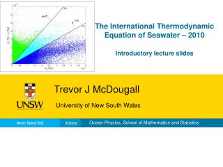
The International Thermodynamic Equation of Seawater – 2010 Introductory lecture slides Trevor J McDougall University of New South Wales Ocean Physics, School of Mathematics and Statistics
These slides provide a short summary of the use of TEOS-10 in oceanography The official guide to TEOS-10 is IOC et al. (2010); the front cover is shown. The www.TEOS-10.org web site serves the computer software, including algorithms to evaluate all the thermodynamic properties of ice and moist air.
Background to TEOS-10 • The 1980 International Equation of State (EOS-80) has served the community very well for 30 years. • EOS-80 provides separate algorithms for density, sound speed, heat capacity and freezing temperature. • However, EOS-80 does not provide expressions for entropy, internal energy and most importantly enthalpy. • All such thermodynamic properties are best derived from a single Gibbs function so that the properties are totally consistent with each other. • The TEOS-10 (Thermodynamic Equation Of Seawater – 2010) Gibbs function incorporates the most recent laboratory data, making the algorithms more accurate, e. g. - the properties of pure water are more accurate than in EOS-80, - the temperature scale has been updated from IPTS-68 to ITS-90. - the density of very cold brackish water is significantly improved.
Features of the new International Thermodynamic Equation of Seawater – 2010 • SCOR/IAPSO Working Group 127 settled on a definition of the Reference Composition of seawater. This was a necessary first step in order to define the Gibbs function at very low salinities. This Reference Composition, consisting of the major components of Standard Seawater, was determined from earlier analytical measurements. • The definition of the Reference Composition enabled the calculation of the Absolute Salinity of seawater that has this Reference Composition (making use of modern atomic weights). • The properties of seawater have been defined up to higher temperatures (80°C; useful for desalination plant design) and to higher Absolute Salinities (120 g kg-1; useful for special places such as Shark Bay, Western Australia).
Solute Mole fraction Mass fraction Chemical Composition of Standard Seawater– the Reference Composition Using the available information and 2005 atomic weight estimates, mole fractions of standard seawater can be determined. The Na+ contribution is determined by the requirement to achieve exact charge balance. The resulting “Reference Composition” is shown to the right. Millero, F. J., R. Feistel, D. G. Wright and T. J. McDougall, 2008: The composition of Standard Seawater and the definition of the Reference-Composition Salinity Scale. Deep-Sea Research I, 55, 50-72.
Reference Salinity as a stepping stone to Absolute Salinity • Practical Salinity is calculated from the conductivity of seawater, and is not the mass fraction of salt in seawater. • The thermodynamic properties of seawater are more closely dependent on the mass fraction (Absolute Salinity SA) of dissolved material, not the conductivity or Practical Salinity SP. • In particular, the density of seawater is a function of SA not of SP. Hence we need to use Absolute Salinity in order to accurately determine the horizontal density gradients (for use in the “thermal wind” equation). • The horizontal density gradient is used via the “thermal wind” equation to deduce the mean ocean circulation. • Hence an accurate evaluation of the ocean’s role in heat transport and in climate change requires the use of Absolute Salinity.
Reference Salinity as a stepping stone to Absolute Salinity • Reference Salinity SR is defined to provide the best available estimate of the Absolute Salinity SA of both (i) seawater of Reference Composition, (ii) Standard Seawater (North Atlantic surface seawater). • SR can be related to Practical Salinity SP (which is based on conductivity ratio) bySR = (35.165 04/35) g kg–1 x SP. • The difference between the new and old salinities of ~0.165 04 g kg–1 (~0.47%) is about 80 times as large as the accuracy with which we can measure SP at sea.
How is the TEOS-10 Gibbs Function used? From a Gibbs function, all of the thermodynamic properties of seawater can be determined by simple differentiation and algebraic manipulation.
Absolute Salinity Anomaly • Practical Salinity SP reflects the conductivity of seawater whereas the thermodynamic properties are more accurately expressed in terms of the concentrations of all the components of sea salt. For example, non-ionic species contribute to density but not to conductivity. • The Gibbs function is expressed in terms of the Absolute Salinity SA (mass fraction of dissolved material) rather than the Practical Salinity SP of seawater. • SA = (35.165 04/35) g kg–1 x SP +
How can we calculate ? • The Absolute Salinity Anomaly is determined by accurately measuring the density of a seawater sample in the laboratory using a vibrating beam densimeter. • This density is compared to the density calculated from the sample’s Practical Salinity to give an estimate of - We have done this to date on 811 seawater samples from around the global ocean. • We exploit a correlation between and the silicate concentration of seawater to arrive at a computer algorithm, a look-up table, to estimateSA = (35.165 04/35) g kg–1 x SP +
This figure is for data from the world ocean below 1000 m. This improvement is mainly due to using SA rather than SP. The red data uses SR in place of SA. Improvement in calculating the horizontal density gradient 60% of the data is improved by more than 2%. improvement in TEOS-10 vs EOS-80 This shows that for calculating density, the other improvementsin TEOS-10 are minor compared with accounting for composition anomalies. Northward density gradient
The North Pacific: 10% change in the thermal wind with TEOS-10 improvement in TEOS-10 vs EOS-80 Northward density gradient
Why adopt Absolute Salinity ? • The pure water content of seawater is [1 – 0.001SA/(g /kg)] not [1 – 0.001SP]. Since SA and SP differ numerically by about 0.47%, there seems no reason for continuing to ignore this difference, for example in ocean models. • Practical Salinity is not an SI unit of concentration. • Practical Salinity is limited to the salinity range 2 to 42. • Density of seawater is a function of SA not of SP. Hence we need to use Absolute Salinity in order to accurately determine the horizontal density gradients (for use in the “thermal wind” equation). • The improved horizontal density gradients will lead to improved heat transports in ocean models.
What is the “heat content” of seawater? • ????? • The air-sea heat flux is a well-defined quantity, and it can be measured. • But what is the heat flux carried by seawater? That is, how would we calculate the meridional heat flux carried by the ocean circulation? • This meridional heat flux is the main role of the ocean in climate and in climate change; but how can we evaluate this heat flux? • ?????
The Ocean’s role in Climate How should we calculate the flux of “heat” through an ocean section?
The concept of potential temperature • Potential temperature, , involves a thought experiment. • You take your seawater sample at pressure p and you mentally put an insulating plastic bag around it, and then you change its pressure. Usually you move the plastic bag to the sea surface where pr = 0 dbar. Once there, you “measure” the temperature and call it “potential temperature”. • In ocean models the air-sea heat flux enters the ocean as a flux of potential temperature, using a constant specific heat capacity.
Present oceanographic practice regarding “heat” To date we oceanographers have treated potential temperature as a conservative variable. We also mix water masses on diagrams as though both salinity and potential temperature are conserved on mixing. In ocean models, air-sea heat fluxes cause a change in using a constant specific heat capacity (whereas in fact varies by 5% at the sea surface). That is, we treat “heat content” as being proportional to • How good are these assumptions? • Can we do better?
The First Law of Thermodynamics in terms of • The First Law of Thermodynamics is written in terms of enthalpy as We would like the bracket here to be a total derivative, for then we would have a variable that would be advected and mixed in the ocean as a conservative variable whose surface flux is the air-sea heat flux. If we take thermodynamic reasoning leads to
Specific heat capacity at constant pressure,cp, J kg-1 K-1 at p = 0 dbar
Potential enthalpy, and Conservative Temperature, • Just as is the temperature evaluated after an adiabatic change in pressure, so potential enthalpy is the enthalpy of a fluid parcel after the same adiabatic change in pressure. Taking the material derivative of this leads to (with ) The “specific heat” is a constant, and the square bracket here is very close to zero, even at a pressure of 40 MPa = 4,000 dbar. This means that the First Law of Thermodynamics can be accurately written as
The difference between potential temperature and Conservative Temperature,
… to be compared with the error in assuming that entropy is a conservative variable; contours in
Improving “Heat” Conservation in Ocean Models • Conservative temperature is 100 times closer to being “heat” than is potential temperature. • The algorithm for conservative temperature has been imported into the MOM4 code and it is available as an option when running the MOM4 code. • The figures show the expected influence of sea-surface temperature in the annual mean, and seasonally.
Improving “Heat” Conservation in Ocean Models • This improvement in the calculation of the “heat content” of seawater and the “heat flux” carried by the ocean circulation is possible because the TEOS-10 Gibbs function delivers the enthalpy of seawater.
The two key changes to oceanographic practice Use of a new salinity variable, Absolute Salinity SA (g/kg) in place of Practical Salinity SP (ocean models need to also keep track of another salinity variable, called Preformed Salinity S*). Use of a new temperature variable, Conservative Temperature replacing potential temperature
The official guide to TEOS-10 is IOC et al. (2010); the front cover is shown. TEOS-10 is the official thermodynamic description of seawater, ice and of humid air at all pressures in the atmosphere. Exploiting the thermodynamic equilibrium properties between seawater, ice and humid air, means that we now have very accurate properties such as freezing temperature, latent heat of evaporation etc.
This short 28-page document is an introduction to TEOS-10 and to the Gibbs Seawater Oceanographic Toolbox of computer algorithms.
Geostrophic Streamfunction for density surfaces The rms error is improved by a factor of 16.
Implementation of TEOS-10 • In October 2008, the International Association for the Properties of Water and Steam (IAPWS) adopted TEOS-10 as the thermodynamic equation of seawater for industrial and engineering purposes. • In June 2009, the Intergovernmental Oceanographic Commission adopted TEOS-10 as the new definition of the thermodynamic properties of seawater in oceanography, effective from 1st January 2010. • The description of TEOS-10 and the TEOS-10 computer software is available at http://www.TEOS-10.org • Oceanographic journals are now encouraging authors to use TEOS-10, including the use of Absolute Salinity. The use of Practical Salinity and EOS-80 in journal articles is being phased out over a transition period (5 years?).
Implementation of TEOS-10 • The thermodynamic properties of seawater are now defined in terms of the TEOS-10 Gibbs function for seawater which is a function of Absolute Salinity. • Continue to report Practical Salinity SP to national data bases since (i) SP is a measured parameter and (ii) we need to maintain continuity in these data bases. • - Note that this treatment of working scientifically with Absolute Salinity but reporting Practical Salinity to national data bases is exactly what we have been doing for temperature; we store in situ temperature, but we have done our research and published in potential temperature.