Download
1 / 53
530 likes | 624 Vues
Learn how to remove objects from images by leveraging information from other images in the set. Explore image rectification, key point detection, and matching using the ASIFT algorithm. Perfect for stock photography, video surveillance, and more.

E N D
Object Removal in Multi-View Photos Aaron McClennon-Sowchuk, MichailGreshischev
Objectives • Remove an object from a set of images by using information (pixels) from other images in the set. • The images mustbe of the same scene but can vary in time of taken and/or perspective of scene. • The allowed variance in time means objects may change location from one image to the next. Applications: stock photography, video surveillance, etc.
Steps • Read Images • Project images in same perspective • Align the images • Identify differences • Infill objects
Reading Images • How are images represented? • Matrices (M x N x P) • M is the width of the image • N is the height of the image • P is 1 or 3 depend on quality of image 1: binary (strictly black/white) or gray-scale images 3: coloured images (3 components of colour: R,G,B) • What tools are capable of processing images? • Many to choose from but MatLab is ideal for matrices. • Hence the name Mat(rix) Lab(oratory)
Object Removal in Multi-View Photos Image Rectification
Image Rectification • Transformation process used to project two-or-more images onto a common image plane. • Corrects image distortion by transforming the image into a standard coordinate system. 1 Figure 1: Example rectification of source images (1) to common image plane (2). 1
Image Rectification To perform a transform... • Cameras are calibrated and provide internal parameters resulting in an essential matrix representingrelationship between the cameras. • We don’t have access to camera’s internal parameters. • What if single camera was used? • The more general case (without camera calibration) is represented by the fundamental matrix. 2
Fundamental Matrix • Algebraic representation of epipolar geometry. • 3×3 matrix which relates corresponding points in stereo images. • 7 degrees of freedom, therefore at least 7 correspondences are required to compute the fundamental matrix. 3
Corresponding Points • Figure out which parts of an image correspond to which parts of another image. • But what is a ‘part’ of an image? • ‘part’ of an image is a Spatial Feature. • Spatial Feature Detection is the process of identifying spatial features in images.
Spatial Feature Detection - Edges • Canny, Prewitt, Sobel, Difference of Gaussians... Figure 2: Example application of Canny Edge Detection 4
Spatial Feature Detection - Corners • Harris, FAST, SUSAN Figure 2: Example application of Harris Corner Detection 5
Feature Description • Simply identifying a feature point is not in itself useful. • consider how one would attempt to match detected feature points between multiple images. • Scale-invariant feature transform (SIFT) offers robust feature description. 6 • Invariant to scale • Invariant to orientation • partially invariant to illumination changes
SIFT • Uses Difference of Gaussians along with multiple smoothing and resampling filters to detect key points (Feature Points with descriptor data) • Key point specifies 2D location, scale, and orientation.
SIFT Figure 3: Sample image for SIFT application. 7
SIFT – Feature Points Figure 4: Detected feature points via SIFT. 7
SIFT – Key Point Figure 5: A SIFT key point in detail. 7
SIFT - Matching • Matches key points by identifying nearest neighbour with the minimum Euclidean distance. • Ensures robustness via... • Cluster identification by Hough transform voting. • Model verification by linear least squares.
SIFT - Matching Figure 5: Example of matched SIFT key points. Note its tolerance to image scale and rotation.
SIFT – Suitable for Multi-View? • SIFT fails to accurately match key points between images which vary significantly in perspective. Figure 7 & 8: Comparison of SIFT accuracy with varying perspective angles. Left image is 45 degrees with 152 matches. Right image is 75 degrees with 11 matches. 8
SIFT – Suitable for Multi-View? • SIFT fails to accurately match key points between images which undergo non-scalable affine transformation or projection. Figure 9: SIFT fails to identify any key point matches between rotated images on a cylinder. 8
ASIFT • Affine-SIFT (ASIFT) is a new framework for fully affine invariant image comparison. • Uses existing SIFT key point descriptors, but matching algorithm has improved.
ASIFT – Improvements over SIFT • Simulated images are compared by a rotation, translation and zoom-invariant algorithm. • (SIFT normalizes translation and rotation and simulates zoom.)
ASIFT – Improvements over SIFT Figure 10: ASIFT (left) identifies 165 matches compared to SIFT’s (right) 11 matches on surface rotated 75 degrees. 8
ASIFT – Improvements over SIFT Figure 10: ASIFT identifies 381 matches between rotated surfaces. 8
Image Rectification • Quick Review... • Given multiple images of the same scene from different perspectives... • We have identified & matched feature points using ASIFT. • We now have sufficient matching points to calculate the fundamental matrix.
Calculating Fundamental Matrix • Random Sample Consensus (RANSAC) is used to eliminate outliers from matched points. • Select 7 points at random. • Use them to compute a Fundamental Matrix between the image pair. • Project every point in the dataset onto the conjugate image pair using the Fundamental Matrix. • If at least 7 points were projected closer to their actual locations than their allowable errors, stop. • Use those 7 points to calculate final Fundamental Matrix.
Example Image Rectification • Input Images
Example Image Rectification • ASIFT Matches
Example Image Rectification • RANSAC selection
Example Image Rectification • Resulting Rectification
Identifying Image Differences • Possible Methods: • Direct subtraction • Structural Similarity Index (SSIM) • Complex Waveform SSIM
Identifying Image Differences • Direct subtraction • Too good to be true! (way too much noise)
Identifying differences • Structural Similarity Index (SSIM) • Number 0-1 indicating how “similar” two pixels are. • 1 indicates perfect match, 0 indicates no similarities at all • Number calculated based on: • Luminance, function of the mean intensity for gray-scale image • Contrast, function of std.dev of intensity for gray-scale image
Object Removal in Multi-View Photos Complex Waveform SSIM
Complex Waveform SSIM • SSIM vs Complex Waveform SSIM(CWSSIM)
CWSSIM - Implementation • Steerable Pyramid constructed for each image • (Steerable Pyramid is a linear multi-scale, multi-orientation image decomposition) • SSIM value calculated for each band, from high to low frequency. • SSIM values for each band are scaled and summed.
CWSSIM - Implementation • Analyzing bands with multi-scale, multi-orientation image decomposition instead of direct pixel comparison provides tolerance for Spatial Shifts. • By reducing the contribution SSIM indexes belonging to high frequency bands we can reduce noise. • …but we lose recognition of changes in that frequency.
CWSSIM - Example • Input Images
CWSSIM - Example • Application of CWSSIM with equal frequency weights.
CWSSIM - Example • Input Images
CWSSIM - Example • Application of CWSSIM with decreased low frequency weight.
Identifying differences • Once again, way too much noise. • SSIM map: 0 black pixel 1 white pixel
Infilling the objects • Concerns: • Identify regions to copy • Calculate a bounding box (smallest area surrounding entire blob) • How to distinguish noise from actual objects? • Area - those blobs with area below threshold are ignored • location - those blobs along an edge of image are ignored. • Copying method • Direct – images from same perspectives • Manipulated pixels – images from different perspectives.
Infilling the objects • Original bounding box results: Matlab returns Left position Top position Width and Height of each box
Infilling the objects • Result with small blobs and blobs along edges ignored: • Left: 119 • Top: 52 • Width: 122 • Height: 264
Infilling the objects • Once regions identified, how can pixels be copied? • Same perspective – direct copy is possible.
Infilling the objects • Result of direct copying
Infilling the objects • Different perspectives • Goal: remove black trophy from left image
Infilling the objects • Direct copying produces horrendous results! Rectified image Result
Work to come... • Copying techniques • Need better method for infilling objects between images in different perspectives. Perhaps use same alignment matrix. • Anti-Aliasing • Method to smooth the edges around pixels copied from one image to another • example looks alright but could improve other test cases • User friendly interface • Current state: a dozen different MatLab scripts. • In the perfect world, we’d have a nice interface to let user load images and clearly displa