Diagonalization
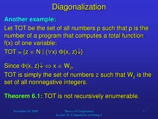
Diagonalization. Another example: Let TOT be the set of all numbers p such that p is the number of a program that computes a total function f(x) of one variable: TOT = {z N | (x) (x, z)} Since (x, z) x W z ,

Diagonalization
E N D
Presentation Transcript
Diagonalization Another example: Let TOT be the set of all numbers p such that p is the number of a program that computes a total function f(x) of one variable: TOT = {z N | (x) (x, z)} Since (x, z) x Wz, TOT is simply the set of numbers z such that Wz is the set of all nonnegative integers. Theorem 6.1: TOT is not recursively enumerable. Theory of Computation Lecture 16: Computation on Strings I
Proof: Suppose that TOT were r.e. Since TOT (we know that there are total unary functions), by Theorem 4.9 there is a computable function g(x) such that TOT = {g(0), g(1), g(2), …}. Let h(x) = (x, g(x)) + 1. Since any g(x) is the number of a program that computes a total function, (x, g(x)) is defined for all x, and h(x) is a computable function. Let h(x) be computed by a program with number p. Then p TOT, which means that p = g(i) for some i. Then h(i) = (i, g(i)) + 1 by definition of h = (i, p) + 1 since p = g(i) = h(i) + 1 since h is computed by p.Contradiction! Diagonalization Theory of Computation Lecture 16: Computation on Strings I
Diagonalization (0, g(0)) (1, g(0)) (2, g(0)) … (0, g(1)) (1, g(1)) (2, g(1)) … (0, g(2)) (1, g(2)) (2, g(2)) … … … … … The elements on the diagonal make it impossible for the function h to be computed by any of the programs g(x). Theory of Computation Lecture 16: Computation on Strings I
Diagonalization Theorem 6.1 gives a reason why we base our studies of computability on partial rather than total functions: By Church’s Thesis, Theorem 6.1 shows that there is no algorithm to determine whether an L program computes a total function. Theory of Computation Lecture 16: Computation on Strings I
Reducibility Another important technique for determining nonrecursive sets is the reducibility method. Once some set (such as the set K) has been shown to be nonrecursive, we can use that set to give other examples of nonrecursive sets. Theory of Computation Lecture 16: Computation on Strings I
Reducibility Definition: Let A, B be sets. Then A is many-one reducible to B, written A m B, if there is a computable function f such that A = {x N | f(x) B}. In other words, x A if and only if f(x) B. “Many-one” means that f does not have to be one-one. If A m B, then testing membership in A is “no harder than” testing membership in B. To test whether x A we can compute f(x) and then test whether f(x) B. Theory of Computation Lecture 16: Computation on Strings I
Reducibility • Theorem 6.2: Suppose A m B. • If B is recursive, then A is recursive. • If B is r.e., then A is r.e. • Proof: Let A = {x N | f(x) B}, where f is computable, and let PB(x) be the characteristic function of B. • Then A = {x N | PB(f(x))}. • If B is recursive, then PB(f(x)), the characteristic function of A, is computable, so A is recursive. • If B is r.e., then B = {x N | g(x)} for some partially computable function g. • Then A = {x N | g(f(x))}, and since g(f(x)) is partially computable, A is r.e. Theory of Computation Lecture 16: Computation on Strings I
Reducibility We will often use Theorem 6.2 in the following form: If A is not recursive (r.e.), then B is not recursive (r.e.). Example: K0 = {z N | r(z)(l(z))} = {x, y | y(x)} Obviously, K0 is r.e. However, we can show that K0 is not recursive by reducing K to K0. K = {n N | n Wn}. Now x K if and only if x, x K0, and the function f(x) = x, x is computable. Therefore, K m K0, and K0 is not recursive. Theory of Computation Lecture 16: Computation on Strings I
Numerical Representation of Strings So far, our programs in the language L have been using natural numbers as their inputs and output. For many applications, however, we would prefer to perform computations on strings on some alphabet instead. You remember that we introduced a numbering of L programs so that L programs could be used as input and output of another (or the same) L program. With regard to strings, we will use the same approach: We will associate numbers with strings on A in a one-one manner. Theory of Computation Lecture 16: Computation on Strings I
Numerical Representation of Strings We will use a system that is very similar to our everyday one-one mapping of natural numbers to strings of digits. There we have a set D of digits, and we define an order s0, …, s9 on these digits: D = {s0, …, s9} = {0, 1, 2, 3, 4, 5, 6, 7, 8, 9}. There are n = 10 elements in our set of digits. Then any string w of digits can be written as w = siksik-1… si1si0, where 0 im n - 1 and k = |w| - 1. Theory of Computation Lecture 16: Computation on Strings I
Numerical Representation of Strings For example, if we have the string w = 372, then k = 2, i2 = 3, i1 = 7, i0 = 2. To find the number associated with this string, we use exactly the following formula: x = iknk + ik-1nk-1 + … + i1n1 + i0n0 x = 3102 + 7101 + 2 = 372. If w = 372 is an octal representation of an integer, then we would have n = 8 and therefore: x = 382 + 781 + 2 = 192 + 56 + 2 = 250 Theory of Computation Lecture 16: Computation on Strings I
Numerical Representation of Strings Now let us develop such a method for strings on an alphabet A. Remember that the set of all strings on an alphabet A, including the empty string, is called A*. Again, let us assume that there is a particular order of symbols in A. We write A = {s1, …, sn} and define that the sequence s1, …, sn corresponds to this order of symbols. Then any string w on A can be written as w = siksik-1… si1, si0, where 1 im n and k = |w| - 1. The empty string is indicated by w = 0. Theory of Computation Lecture 16: Computation on Strings I
Numerical Representation of Strings Then we use exactly the same formula as before to associate w with an integer x: x = iknk + ik-1nk-1 + … + i1n1 + i0n0 . With w = 0 we associate the number x = 0. For example, consider the alphabet A = {a, b, c} and the string w = caba. Then x = 333 + 132 + 231 + 1 = 81 + 9 + 6 + 1= 97. Now why is this representation unique? We can prove this by showing how to retrieve the subscripts i0, i1, …, ik from x for any x > 0. Theory of Computation Lecture 16: Computation on Strings I