Download

1 / 40
410 likes | 594 Vues
An ALM Linear Stochastic Programming Model for a Brazilian pension fund. Presenter Davi Michel Valladão Pontifícia Universidade Católica do Rio de Janeiro - Brazil davi_michel@yahoo.com.br Co-authors Álvaro de Lima Veiga Filho, PUC-Rio Ana Tereza Vasconcellos Estellita Pessoa, PUC-Rio

E N D
An ALM Linear Stochastic Programming Model for a Brazilian pension fund Presenter Davi Michel Valladão Pontifícia Universidade Católica do Rio de Janeiro - Brazil davi_michel@yahoo.com.br Co-authors Álvaro de Lima Veiga Filho, PUC-Rio Ana Tereza Vasconcellos Estellita Pessoa, PUC-Rio Camila Spinassé, PUC-Rio
Summary • Motivation • Asset • Liability • Optimization • Illustration • Conclusion and future works
Motivation • ALM • Linear Stochastic Programming • Literature • Model General Description
ALM ALM Markowitz Multi-period solution Scenario tree structure Linear stochastic programming One-period solution Mean-variance model Quadratic programming • Asset and Liability Management • Definition: It is process of strategic formulation, implementation and revision of investments and liabilities to reach the institutional financial goals given some restrictions.
Linear Programming Deterministic Stochastic Known asset returns Known liability cash flows Optimization problem: max c.x s.t. A.x=b Stochastic returns Unknown liability cash flows Scenario tree structure Optimization problem: max E[c.x] s.t. Ai.x=b , i=1,..N
Literature • Drijver, Klein and Vlerk – OR, 2000 • Scenario tree generation • Cost of funding minimization • Chance constraint and transaction costs • Kouwenberg – OR, 2001 • Scenario tree generation • Cost of funding minimization • Maximum allocation constraints and transaction costs • Hilli, Koivu and Pennanen – OR, 2004 • Scenario tree generation • Maximum expected wealth utility • Maximum allocation constraints, transaction costs and regulatory constraints • Gulpinar, Rustem and Settergren – JEDC, 2004 • Scenario tree generation – methods comparison
Model General Description • Strategic allocation indexes instead of assets • Long run (20 years) • asset classes: stocks, interest rate, inflation • Scenario tree generation • Maximum final wealth with underfunding penalty • Transaction costs • Regulatory constraints (Brazilian law) • Liquidity constraints
Model General Description Stochastic forecast of economic variables Stochastic asset returns Optimization Model Asset Scenario Generation VAR Model Optimal Allocation Inflation Scenarios Stochastic nominal cash flow Deterministic real cash flow Liability Scenario Generation Liability Model
Asset • VAR Model • Scenario Tree Generation
VAR Model • Based on Brazil’s Central Bank working paper number 33 (Minella – RBE, 2003) • A, B, C and S estimated with past data *All series computed as log first difference
VAR Model • Estimated coefficients
VAR Model • Estimated coefficients
VAR Model • Estimated coefficients
VAR Model • Estimated coefficients
VAR Model • Residual Normality test
VAR Model • Residual serial correlation test
VAR Model • Impulse Response
Scenario Tree Generation • Tree Structure: 1-10-6-6-4-4 … 4X Yt = A + B.Yt-1 + C.Yt-2 + et(j) … 4X … 6X Adjusted Random Sampling … 6X ………………..… ………….… ……… … … 10X … 6X … 6X Initial Allocation … 4X … 4X 1 year 1 year 3 year 5 year 10 year t (10 branches) (60 branches) (360 branches) (1440 branches) (5760 branches)
Scenario Tree Generation • Adjusted Random Sampling (Kouwenberg – OR,2001) • For each root or branch node: • Generate k/2 values of et(j) , j=1,… k/2 • Compute antithetic values: et(j + k/2) = - et(j) • Variance adjustment for each tree stage et(j)*[Std. dev.(VAR)/Std. dev.(et(j ))], j=1,…k • Compute:Yt = A + B.Yt-1 + C.Yt-2 + et(j)
Liability • Liability Model • Liability Scenario Generation
Liability Model • Artificial data • Defined benefit plan • No new participants • Risk factors • Mortality • Retirement time • Monte Carlo Simulation • Deterministic output (simulation average real value)
Liability Scenario Generation • Input: • Deterministic real cash flows • Inflation scenarios (new risk factor included) • Output: • Stochastic Nominal cash flows
Optimization Model • Objective Function • Constraints
Objective function “Maximize the expected final wealth with underfunding penalty” • prob[N] = scenario N probability • y[N] = wealth at the end of the studied period (scenario N) • w[N] = deficit at the end of the studied period (scenario N) • b = bonus • p = penalization
Constraints • For each pair of linked nodes (A,B), there are the following constraints • Balance • Transaction … B … A … … … … … … • Liquidity • Maximum allocation on stocks (regulatory)
Constraints • Balance constraints • xi (N) = value ($) in asset i at node N • ri = asset i return • L = liability nominal cash flow • TC = Transaction cost
Constraints • Balance constraints (for B as a final node) • xi (N) = value ($) in asset i at node N • ri = asset i return • L = liability nominal cash flow • TC = Transaction cost • y[N] = wealth at the end of the studied period (scenario N) • w[N] = deficit at the end of the studied period (scenario N)
Constraints • Transaction constraints • Liquidity constraint • buyi (N)= how much was bought from asset i at node N • selli (N)= how much was sold from asset i at node N
Illustration • Assumptions • Deficit Probability X Initial Wealth • Liquidity Problem X Initial Wealth • Transaction costs X Initial Wealth • Optimal Initial Allocation X Initial Wealth • Optimal Expected Allocation
Assumptions • Based on one of the most important sponsored pension fund in Brazil • 161 thousands lives simulated • 83 thousands active participants • 59 thousands retired participants • 19 thousands pensioners • Standard family concept • Real wage growth: 2% per year • Contribution: 16% of wage (8% from participant and 8% from sponsor) • Benefit: 90% of the wage average of the last 12 months
Deficit Probability X Initial Wealth Related wealth Deficit level 100% = 44 billions of dollars
Liquidity Problem X Initial Wealth 100% = 44 billions of dollars
Conclusion and Future Works • ALM is an important decision instrument (not exploited in Brazil) • Model characteristic: • Linear Stochastic Programming • Transaction cost and Brazilian law incorporated • Liquidity problem included • Future works • Check VEC Model for economic variables • Include end-effects • Make a Stochastic liability model • Use Wage as risk factor