Capital Structure Management in Practice
13. Capital Structure Management in Practice. Introduction. This chapter focuses on tools of analysis that can assist managers in making capital structure decisions that will lead to a maximization of shareholder wealth.

Capital Structure Management in Practice
E N D
Presentation Transcript
13 Capital Structure Management in Practice
Introduction • This chapter focuses on tools of analysis that can assist managers in making capital structure decisions that will lead to a maximization of shareholder wealth. • It develops techniques, derived from accounting data, for measuring operating and financial leverage.
Operating and Financial Leverage • Leverage • A firm’s use of assets and liabilities having fixed costs in an attempt to increase potential returns to stockholders • Operating leverage • The use of assets having fixed costs • Financial leverage • The use of liabilities (and preferred stock) having fixed costs
Various Categories of Costs • From fixed operating or fixed capital costs • Operating costs • Costs of sales • General, administrative, and selling expenses • Capital costs • Interest charges • Preferred dividends • Income taxes
Short-Run Costs • Over the short run, certain operating costs within a firm vary directly with the level of sales whereas other costs remain constant, regardless of changes in the sales level. Costs that move in close relationship to changes in sales are called variable costs.
Short-Run Costs • Variable costs are tied to the number of units produced and sold by the firm, rather than to the passage of time. They include raw material and direct labor costs, as well as sales commissions.
Short-Run Costs • Over the short run, certain other operating costs are independent of sales or output levels. These, termed fixed costs, are primarily related to the passage of time. Depreciation on property, plant, and equipment; rent; insurance; lighting and heating bills; property taxes; and the salaries of management are all usually considered fixed costs.
Short-Run Costs • If a firm expects to keep functioning, it must continue to pay these fixed costs, regardless of the sales level.
Short-Run Costs • A third category, semivariable costs, can also be considered. Semivariable costs are costs that increase in a stepwise manner as output is increased. One cost that sometimes behaves in a stepwise manner is management salaries.
Short-Run Costs • Whereas semivariable costs are generally considered fixed, this assumption is not always valid. A firm faced with declining sales and profits during an economic downturn may often cut the size of its managerial staff.
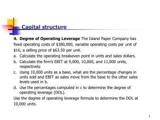
Short-Run Costs • Panels (a), (b), and (c) of Figure 13.1 show the behavior of variable, fixed, and semivariable costs, respectively, over the firm’s output range.
Long-Run Costs • Over the long run, all costs are variable. In time, a firm can change the size of its physical facilities and number of management personnel in response to changes in the level of sales. Fixed capital costs also can be changed in the long run.
Operating and Financial Leverage • Operating leverage has fixed operating costs for its “fulcrum.” When a firm incurs fixed operating costs, a change in sales revenue is magnified into a relatively larger change in earnings before interest and taxes (EBIT). The multiplier effect resulting from the use of fixed operating costs is known as the degree of operating leverage.
Operating and Financial Leverage • Financial leverage has fixed capital costs for its “fulcrum.” When a firm incurs fixed capital costs, a change in EBIT is magnified into a larger change in earnings per share (EPS). The multiplier effect resulting from the use of fixed capital costs is known as the degree of financial leverage.
% Sales DOL % EBIT DFL % EPS Leverage Model
Degree of Operating Leverage • A firm’s degree of operating leverage (DOL) is defined as the multiplier effect resulting from the firm’s use of fixed operating costs. More specifically, DOL can be computed as the percentage change in earnings before interest and taxes (EBIT) resulting from a given percentage change in sales (output):
Degree of Operating Leverage • The formula in the previous slide can be rewritten as follows (13.1): where ΔEBIT and ΔSales are the changes in the firm’s EBIT and sales, respectively.
Degree of Operating Leverage • Because a firm’s DOL differs at each sales (output) level, it is necessary to indicate the sales (units of output or dollar sales) point X, at which operating leverage is measured.
Degree of Operating Leverage • The degree of operating leverage is analogous to the elasticity concept of economics (for example, price and income elasticity) in that it relates percentage changes in one variable (EBIT) to percentage changes in another variable (sales).
Degree of Operating Leverage • The calculation of the DOL can be illustrated using the Allegan Manufacturing Company example in Table 13.1. Since Allegan’s variable operating costs were $3 million at the current sales level of $5 million. Therefore, the firm’s variable operating cost ratio is ($3 million)/($5 million) = 0.60, or 60 percent.
Degree of Operating Leverage • Suppose the firm increased sales by 10 percent to $5.5 million while keeping fixed operating costs constant at $1 million and the variable (operating) cost ratio at 60 percent. As can be seen in Table 13.2, this would increase the firm’s earnings before interest and taxes (EBIT) to $1.2 million.
Degree of Operating Leverage • Substituting the two sales figures ($5 million and $5.5 million) and associated EBIT figures ($1 million and $1.2 million) into equation yields the following:
Degree of Operating Leverage • A DOL of 2.0 is interpreted to mean that each 1 percent change in sales from a base sales level of $5 million results in a 2 percent change in EBIT in the same direction as the sales change. In other words, a sales increase of 10 percent results in a 20% increase in EBIT. Similarly, a 10 percent decrease in sales produces a 20% decrease in EBIT.
Degree of Operating Leverage • The greater a firm’s DOL, the greater the magnification of sales changes into EBIT changes.
Degree of Operating Leverage • Another equation that can be used to compute a firm’s DOL more easily is Equation (13.2) as follows: • Note: EBIT = Sales – Variable costs – Fixed costs
Degree of Operating Leverage • Inserting data from Table 13.1 on the Allegan Manufacturing Company into Equation (13.2) gives the following: This result is the same as that obtained using the more complex Equation (13.1).
Degree of Operating Leverage • Table 13.3 shows the DOL at various sales levels for Allegan Mangan Manufacturing Company. Note that Allegan’s DOL is largest (in absolute value terms) when the firm is operating at the break-even sales point [that is, where Sales = $2,500,000 and EBIT = Sales – Variable Operating Costs – Fixed Operating Costs = $2,500,000 – 0.6($2,500,000) – $1,000,000 = $0].
Degree of Operating Leverage • Note also that the firm’s DOL is negative below the break-even sales level. A negative DOL indicates the percentage reduction in operating losses that occurs at the result of a 1 percent increase in output. For example, the DOL of -1.50 at a sales level of $1,500,000 indicates that, from a base sales level of $1,500,000, the firm’s operating losses are reduced by 1.5 percent for each 1 percent increase in output.
Degree of Operating Leverage • A firm’s DOL is a function of the nature of the production process. If the firm employs large amounts of labor-saving equipment in its operations, it tends to have relatively high fixed operating costs and relatively low variable operating costs. Such a cost structure yields a high DOL, which results in large operating profits (positive EBIT) if sales are high and large operating losses (negative EBIT) if sales are depressed.
Degree of Financial Leverage • A firm’s degree of financial leverage (DFL) is computed as the percentage change in earnings per share (EPS) resulting from a given percentage change in earnings before interest and taxes (EBIT):
Degree of Financial Leverage • The formula in the previous slide can also be written as Equation (13.3) as follows: where ΔEPS and ΔEBIT are the changes in EPS and EBIT, respectively.
Degree of Financial Leverage • Because a firm’s DFL is different at each EBIT level, it is necessary to indicate the EBIT point, X, at which financial leverage is being measured.
Degree of Financial Leverage • Using the information contained in Table 13.4 and shown in Figure 13.2, the degree of financial leverage used by the Allegan Manufacturing Company can be calculated. The firm’s EPS level is $3.00 at an EBIT level of $1 million. At an EBIT level of $1.2 million, EPS equals $4.20. Substituting these quantities into the Equation yields the following:
Degree of Financial Leverage A DFL of 2.0 indicates that each 1 percent change in EBIT from a base EBIT level of $1 million results in a 2 percent change in EPS in the same direction as the EBIT change.
Degree of Financial Leverage • The formula of DFL can also be rewritten as follows (13.4): where I is the firm’s interest payments, Dp the firm’s preferred dividend payments, T the firm’s marginal income tax rate, and X the level of EBIT at which the firm’s DFL is being measured.
Degree of Financial Leverage • For the firm with no preferred stock, Equation (13.4) becomes the following: where EBT represents earnings before taxes.
Degree of Financial Leverage • Unlike interest payments, preferred dividend payments are not tax deductible. Therefore, on a comparable tax basis, a dollar of preferred dividends costs the firm more than a dollar of interest payments. Dividing preferred dividends in Equation (13.4) by (1 – T) puts interest and preferred dividends on an equivalent, pretax basis.
Degree of Financial Leverage • As shown in Figure 13.2, Allegan will have EPS = $0 at an EBIT level of $500,000. With this level of EBIT, there is just enough operating earnings to pay interest ($250,000) and preferred dividends (after-tax). Using the Equation (13.4), it can be seen that DFL will be maximized at that level of EBIT where EPS = 0.
Degree of Financial Leverage • Consider again the data presented in Table 13.1 on the Allegan Manufacturing Company. According to that table, EBIT = $1 million, I= $250,000, Dp = $150,000, and T = 40 percent, or 0.40.
Degree of Financial Leverage • Substituting these values into the Equation (13.4) yields the following: This result is the same as that obtained using Equation (13.3).
Degree of Financial Leverage • Just as a firm can change its DOL by raising or lowering fixed operating costs, it can also change its DFL by increasing or decreasing fixed capital costs. The amount of fixed capital costs incurred by a firm depends primarily on the mix of debt, preferred stock, and common stock equity in the firm’s capital structure.
Degree of Financial Leverage • Thus, a firm that has a relatively large proportion of debt and preferred stock in its capital structure will have relatively large fixed capital costs and a high DFL.
Degree of Combined Leverage • Combined leverage occurs whenever a firm employs both operating leverage and financial leverage in an effort to increase the returns to common stockholders.
Degree of Combined Leverage • Combined leverage represents the magnification of sales increases (or decreases) into relatively larger earnings per share increases (or decreases), resulting from the firm’s use of both types of leverage. The joint multiplier effect is known as the degree of combined leverage.
Degree of Combined Leverage • A firm’s degree of combined leverage (DCL) is computed as the percentage change in earnings per share resulting from a given percentage change in sales: