Exploring Relationships Between Variables with Scatterplots and Regression
400 likes | 487 Vues
Delve into examining links between two variables through scatterplots, correlation measures like r, regression lines, and prediction methods, uncovering nuances in associations for more accurate interpretations.

Exploring Relationships Between Variables with Scatterplots and Regression
E N D
Presentation Transcript
Chapter 3Association: Contingency, Correlation, and Regression • Learn …. How to examine links between two variables
Section 3.2 How Can We Explore the Association Between Two Quantitative Variables?
Scatterplot • Graphical display of two quantitative variables: • Horizontal Axis: Explanatory variable, x • Vertical Axis: Response variable, y
Positive Association • Two quantitative variables, x and y, are said to have a positive association when high values of x tend to occur with high values of y, and when low values of x tend to occur with low values of y
Negative Association • Two quantitative variables, x and y, are said to have a negative association when high values of x tend to occur with low values of y, and when low values of x tend to occur with high values of y
Example: Did the Butterfly Ballot Cost Al Gore the 2000 Presidential Election?
Linear Correlation: r • Measures the strength of the linear association between x and y • A positive r-value indicates a positive association • A negative r-value indicates a negative association • An r-value close to +1 or -1 indicates a strong linear association • An r-value close to 0 indicates a weak association
Example: 100 cars on the lot of a used-car dealership Would you expect a positive association, a negative association or no association between the age of the car and the mileage on the odometer? • Positive association • Negative association • No association
Section 3.3 How Can We Predict the Outcome of a Variable?
Regression Line • Predicts the value for the response variable, y, as a straight-line function of the value of the explanatory variable, x
Example: How Can Anthropologists Predict Height Using Human Remains? • Regression Equation: • is the predicted height and is the length of a femur (thighbone), measured in centimeters
Example: How Can Anthropologists Predict Height Using Human Remains? • Use the regression equation to predict the height of a person whose femur length was 50 centimeters
Interpreting the y-Intercept • y-Intercept: • the predicted value for y when x = 0 • helps in plotting the line • May not have any interpretative value if no observations had x values near 0
Interpreting the Slope • Slope: measures the change in the predicted variable for every unit change in the explanatory variable • Example: A 1 cm increase in femur length results in a 2.4 cm increase in predicted height
Residuals • Measure the size of the prediction errors • Each observation has a residual • Calculation for each residual:
Residuals • A large residual indicates an unusual observation • Large residuals can easily be found by constructing a histogram of the residuals
“Least Squares Method” Yields the Regression Line • Residual sum of squares: • The optimal line through the data is the line that minimizes the residual sum of squares
Regression Formulas for y-Intercept and Slope • Slope: • Y-Intercept:
The Slope and the Correlation • Correlation: • Describes the strength of the association between 2 variables • Does not change when the units of measurement change • It is not necessary to identify which variable is the response and which is the explanatory
The Slope and the Correlation • Slope: • Numerical value depends on the units used to measure the variables • Does not tell us whether the association is strong or weak • The two variables must be identified as response and explanatory variables • The regression equation can be used to predict the response variable
Section 3.4 What Are Some Cautions in Analyzing Associations?
Extrapolation • Extrapolation: Using a regression line to predict y-values for x-values outside the observed range of the data • Riskier the farther we move from the range of the given x-values • There is no guarantee that the relationship will have the same trend outside the range of x-values
Regression Outliers • Construct a scatterplot • Search for data points that are well removed from the trend that the rest of the data points follow
Influential Observation • An observation that has a large effect on the regression analysis • Two conditions must hold for an observation to be influential: • Its x-value is relatively low or high compared to the rest of the data • It is a regression outlier, falling quite far from the trend that the rest of the data follow
Correlation does not Imply Causation • A correlation between x and y means that there is a linear trend that exists between the two variables • A correlation between x and y, does not mean that x causes y
Lurking Variable • A lurking variable is a variable, usually unobserved, that influences the association between the variables of primary interest
Simpson’s Paradox • The direction of an association between two variables can change after we include a third variable and analyze the data at separate levels of that variable
Example: Is Smoking Actually Beneficial to Your Health? • An association can look quite different after adjusting for the effect of a third variable by grouping the data according to the values of the third variable
Data are available for all fires in Chicago last year on x = number of firefighters at the fires and y = cost of damages due to fire Would you expect the correlation to be negative, zero, or positive? • Negative • Zero • Positive
Data are available for all fires in Chicago last year on x = number of firefighters at the fires and y = cost of damages due to fire If the correlation is positive, does this mean that having more firefighters at a fire causes the damages to be worse? • Yes • No
Data are available for all fires in Chicago last year on x = number of firefighters at the fires and y = cost of damages due to fire Identify a third variable that could be considered a common cause of x and y: • Distance from the fire station • Intensity of the fire • Time of day that the fire was discovered