Download
1 / 72
720 likes | 855 Vues
Get physics under control Magnitude of force of gravity. Notice from symmetry is 1-D problem. 2) Get MATLAB under control g is a vector in this case we will only need 2-d vectors (from symmetry) so we need a way to represent vectors

E N D
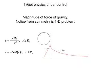
Get physics under control Magnitude of force of gravity. Notice from symmetry is 1-D problem.
2) Get MATLAB under control g is a vector in this case we will only need 2-d vectors (from symmetry) so we need a way to represent vectors For the case of 2-d vectors MATLAB has two ways to represent vectors Use regular MATLAB vectors [a], [b], or [a,b] Use complex numbers a+ib
It turns out that MATLAB does some interesting things with complex numbers and it is easier to use the complex number method when you can.
MATLAB (usually, sometimes?) treats a vector of complex numbers as a vector of [x,y] pairs. For instance >> x=[0:5] x = 0 1 2 3 4 5 >> z=x+i*x.^2 z = Columns 1 through 5 0 1.0000 + 1.0000i 2.0000 + 4.0000i 3.0000 + 9.0000i 4.0000 +16.0000i Column 6 5.0000 +25.0000i >> plot(z)
To calculate the force of gravity on the surface of a homogeneous earth we will need to calculate gravity on a set of points on a circle with the radius of the earth.
Consider the following line of code c= exp((0:N)*pi*2i/(N-1)); What does this do? (notice that I don’t need 2*i MATLAB does not allow variables that start with numbers so it can figure this out.
So now we have a MATLAB vector of complex numbers that defines a circle centered on the origin. and Let’s call each of the [x,y] pairs represented by the complex number x+iy a Physics vector.
I’ll use the term MATLAB vectors (“matrices”) for collections of things into “vectors” (“matrices”) that do not represent things in the physics but make the organization and calculations of the program easier and I’ll use the term Physics vectors for things that represent components of the physics and geometry.
Applying our definitions to the results of the line of code c= exp((0:N)*pi*2i/(N-1)); We get a MATLAB vector c that is a collection of Physical vectors (the vectors from the origin to the points of a circle about the origin).
We have to calculate gravity (a Physics vector - magnitude and direction) at each of these points. How do we get the direction of gravity? For the homogeneous earth, the force of gravity is directed radially inward.
We can calculate the angle q, which is the normal to the circle, from tan-1(y/x).
But we really want a Physics vector [gx, gy] at the point [x,y] (another Physics vector), not the angle q. Consider the line of code vc=c./abs(c); What does this do?
The MATLAB vector vc contains the unit (Physics) vectors (for a vector from the origin to a point on the circle) at each of the points in c.
Lets plot it up to see what we have Use quiver to plot vector field. Quiver needs the positions (which we have in the vector c) of Physics vectors and the components of the Physics vectors (which we have in the vector vc of unit vectors) quiver(x,y,u,v). Unfortunately quiver does not work with the complex number to [x,y] vector trick, so you need to pass it MATLAB vectors of x, y, u and v.
Lets plot it up to see what we have (don’t plot all of them – use estep to decimate, do vectors twice, once times -1 to get both outward and inward normals) Have to pull out real and imag parts for quiver. %linespec of "." gets rid of arrow head on quiver!! quiver(real(c(1:estep:end)),imag(c(1:estep:end)),real(vc(1:estep:end)),imag(vc(1:estep:end)),'.r') axis equal hold quiver(real(c(1:estep:end)),imag(c(1:estep:end)),-real(vc(1:estep:end)),-imag(vc(1:estep:end)),'.r') plot(c) plot(0+i*0,'+r') grid
That was amazingly easy. The calculations took all of 2 lines of code! There was much more code to plot it than calculate it!!
So we have basically plotted g on the surface of the earth. Since g is radial and has uniform magnitude on the surface of a homogeneous sphere – all we have to do is state the scale and we are done [if we drew only the inward pointing vectors and left the arrow head on them].
What about for the anomaly? We now need Physics vectors that go from the center of the anomaly to the surface of the earth. We have a MATLAB vector with the physics vectors from the center of the earth to each point on the surface.
What about for the anomaly? The center of the anomaly is at [0,ca] or i*ca so we can make a new MATLAB vector of the Physics vectors from the center of the anomaly to the surface of the earth ac=c-i*ca using vector addition (both MATLAB and Physics simultaneously)
What about for the anomaly? And we find the unit vectors on the circles representing both the anomaly and the surface of the earth from vca=ac./abs(ac) using vector addition and multiplication (both MATLAB and Physics simultaneously)
So, in another 2 lines of code we have the Physics vectors on the surface of the earth that are the radials of the anomaly
To make this plot I took my circle, c, of unit radius and multiplied/scaled it by the radius of the earth to make the big circle (one line a code – a multiply). I then took my unit circle, c, again and scaled it by the radius of the anomaly (one line of code, a multiply) and then offset it to the position of the anomaly (one line of code, an add).
I then plotted both circles. I next used quiver to draw the vectors from the center of the anomaly to the surface of the earth (twice to get the outward in inward vectors)
You can easily see that the vectors are normal to the surface of the anomaly (as expected) So far we have not calculated the magnitude, which in this case, as opposed to the previous case for the earth, vary as a function of position on the surface of the earth.
So how do we calculate the magnitude of the gravity due to the anomaly on the surface of the earth. We have a MATLAB vector with the Physics vectors from the center of the anomaly to the surface of the earth (vector ac).
We are outside the anomaly so the magnitude of g is g=-GMa/r2 So the magnitude of g is gsea=-G*ma./abs(ac).^2; (we could have also done ac*ac’ in the denom.) Where we are using MATLAB and Physics vectors simultaneously.
To get the Physical vector g we just multiply the MATLAB vector of magnitudes by the MATLAB vector of (Physics) unit vectors element by element. gseav=gsea.*vca; So gseav is a MATLAB vector, where each element is a Physics vector.
Plotting this up we get g on the surface of the earth from the anomaly.
Using superposition, to get the total force of gravity on the surface of the earth (from the earth and the anomaly) one adds the Physics vectors (and you do this for the whole set of points on the surface of the earth at once by adding the two MATLAB vectors) Note that it is very important to add them as vectors – not just the magnitudes
By representing the physical vectors (the ones from the centers of the earth and anomaly to the surface, g, etc.) as complex numbers we were able to use MATLAB vectors to hold our sets of physical vectors (x,y)=x+iy, magnitudes, and unit vectors. We used simple scaling and shifting to make the earth and anomaly from a single unit circle. We used regular vector arithmetic (combined use of MATLAB and Physics vectors into one step) to do this.
By representing the physical vectors (the ones from the centers of the earth and anomaly to the surface, g, etc.) as complex numbers we were able to use MATLAB vectors to hold our sets of physical vectors We were able to organize our code based on the Physics (two simple gravity fields and add them together), rather than the details of index bookeeping (as would be necessary in fortran). The code is easier to understand and follow (especially if you need to maintain it/look at it in 6 months).
Now we are ready to attack the problem of calculating g everywhere in a plane that goes through the symmetry axis.
First we have to make our sampling grid. Use the MATLAB routine meshgrid [xeg,yeg]=meshgrid([-maxp:step:maxp]); Which produces two MATLAB matricies – one with the x values and one with the y values for our grid. So any point on the grid is x(m,n), y(m,n).
How are we going to “fix” this to get our Physics vectors to each point?
How about xyegrd=xeg+i*yeg; To make a MATLAB matrix of Physics vectors to each point.
And then dce=abs(xyegrd); To get the distance from the origin (center of earth) to each point. and vxyegrd=xyegrd./dce; To get the unit vector direction at each point.
Now we just repeat what we did before. With one difference. We now have to take into account whether or not we are inside or outside the earth or anomaly.
What do we want to do? We have a matrix that has the position of each point where we would like to calculate gravity. We have a matrix that has the distance from the center of the earth to each point. Each (p,q) element of first matrix is paired to the (p,q) element of the second matrix, they “go” together. We would like to create 2 new matrices that have 1) the magnitude and 2) the direction of gravity at each point, with the same pairing of elements.
MATLAB again comes to the rescue. Consider the lines of code ge=dce; ge(dce>re)=-G*me./dce(dce>re).^2; What does this do?
ge=dce; ge(dce>re)=-G*me./dce(dce>re).^2; How it works is not intuitively obvious.
Start with small example The line “test a>=4” returns a logical matrix whose elements are logicals that contain the results of the test on each element of the matrix (1 for true, 0 for false). >> a=magic(3) a = 8 1 6 3 5 7 4 9 2 >> a>=4 ans = 1 0 1 0 1 1 1 1 0 >> whos Name Size Bytes Class Attributes a 3x3 72 double ans 3x3 9 logical
>> a=magic(3) a = 8 1 6 3 5 7 4 9 2 >> a>=4 ans = 1 0 1 0 1 1 1 1 0 >> a(a>=4) ans = 8 4 5 9 6 7 >> How can we use this? MATLAB has a feature called “logical indexing” in which it uses a logical array for the matrix subscript and returns the elements for which the logical array value is true. It returns these elements in a column vector (1-D, linear index).
>> a a = 8 1 6 3 5 7 4 9 2 >> find(a>4) ans= 1 5 6 7 8 >> a(:) ans= 8 3 4 1 5 9 6 7 2 >> If you want to explicitly identify the elements in “a” that meet the test, use the MATLAB find command. Note that it returns a vector with a linear index into the matrix (the line a(:) shows how the elements of a are stored in memory as a 1-d vector).
Note that the logical array has to be the same size or smaller than the array being tested (it goes through both using linear indexing till the logical array runs out of elements). (This is true in this case since the same matrix, a, is being tested and was used to generate the logical array. In our gravity example, however, we are using two different arrays on the LHS.) >> a=magic(3) a = 8 1 6 3 5 7 4 9 2 >> a>=4 ans = 1 0 1 0 1 1 1 1 0 >> a(a>=4) ans = 8 4 5 9 6 7 >>
This is not quite what we need, since the result is a column vector and we don’t know where these elements came from in the original array. Remember that the element position (m,n) in the original arrays map into the geometry and physics of the problem (the position and value of the variable). So we need a way to maintain the original indexing in a. >> a=magic(3) a = 8 1 6 3 5 7 4 9 2 >> a>=4 ans = 1 0 1 0 1 1 1 1 0 >> a(a>=4) ans = 8 4 5 9 6 7 >>
>> a=magic(3) a = 8 1 6 3 5 7 4 9 2 >> a>=4 ans = 1 0 1 0 1 1 1 1 0 >> b=zeros(3); >> b(a>=4)=a(a>=4) b= 8 0 6 0 5 7 4 9 0 >> Use the same scheme on the LHS. Put the elements selected on the RHS into the elements selected on the LHS.
>> a=magic(3) a = 8 1 6 3 5 7 4 9 2 >> b=zeros(3); >> b(a>=4)=a(a>=4) b= 8 0 6 0 5 7 4 9 0 >> >> b=zeros(2); >> b(ind)=a(ind) ??? In an assignment A(I) = B, a matrix A cannot be resized. >> b=zeros(1,8); >> b(ind)=a(ind) b= 8 0 0 0 5 9 6 7 >> b=zeros(8,1); >> b(ind)=a(ind) b= 8 0 0 0 5 9 6 7 >> Note that “b” has to be big enough to hold all the elements that come from the RHS (which is not the number of elements in “a” on the RHS [9] but the number needed to go from the start of “a” to the last value that meets the condition [8]. (If we used a<4 it would have put out 9 elements since the last element in “a” meets the condition).