Download
1 / 43
440 likes | 626 Vues
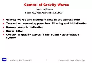
Control of Gravity Waves. Lars Isaksen Room 308, Data Assimilation, ECMWF. Gravity waves and divergent flow in the atmosphere Two noise removal approaches: filtering and initialization Normal mode initialization Digital filter Control of gravity waves in the ECMWF assimilation system.

E N D
Control of Gravity Waves Lars Isaksen Room 308, Data Assimilation, ECMWF • Gravity waves and divergent flow in the atmosphere • Two noise removal approaches: filtering and initialization • Normal mode initialization • Digital filter • Control of gravity waves in the ECMWF assimilation system
Processes and waves in the atmosphere • Sound waves, synoptic scale waves, gravity waves, turbulence, Brownian motions .. • The atmospheric flow is quasi-geostrophic and largely rotational (non-divergent) – mass/wind balance at extra-tropical latitudes • The energy in the atmosphere is mainly associated with fairly slow moving large-scale and synoptic scale waves (Rossby waves) • Energy associated with gravity waves is quickly dissipated/dispersed to larger scale Rossby waves: the quasi-geostrophic balance is reinstated
500 hPa Geopotential height and winds Approximate mass-wind balance
MSL pressure and 10 metre winds Approximate mass-wind balance
Which atmospheric processes/waves are important in data assimilation and NWP? • Sound and gravity waves are generally NOT important, but can rather be considered a nuisance • Fast waves in the NWP system require unnecessary short time steps – inefficient use of computer time • Large amplitude gravity waves add high frequency noise to the assimilation system resulting in: • rejection of correct observations • noisy forecasts with e.g. unrealistic precipitation • BUT certain gravity waves and divergent features should be retained in a realistic assimilation system. We will now present some examples.
Ageostrophic motion – Jet stream related An important unbalanced synoptic feature in the atmosphere Wind and height fields at 250 hPa Ageostrophic winds at 250 hPa
Mountain generated gravity waves should be retained Rocky Mountains
Temperature cross-section over Norway Gravity waves in the ECMWF analysis Pressure [hPa] Acknowledgements to Agathe Untch Norway
Analysis temperatures at 30 hPa Acknowledgements to Agathe Untch
Divergent winds at 150hPa: ERA-40 average March 1989 Acknowledgements to Per Kållberg
Observed Mean Sea-Level pressure - Tropics Semi-diurnal tidal signal for Seychelles (5N 56E)
Filtering the governing equations • Quasi-geostrophic equations/ omega equation • Primitive equations with hydrostatic balance • Primitive equations with damping time-step like Eulerian backward • Primitive equations with digital filter Goal: Use filtered model equations that do not allow high frequency solutions (“noise”) – but still retain the “signal”
Initialization Goal: Remove the components of the initial field that are responsible for the “noise” – but retain the “signal” • Make the initial fields satisfy a balance equation, e.g. quasi-geostrophic balance or • Set tendencies of gravity waves to zero in initial fields – Non-linear Normal Mode Initialization
Normal-mode initialization Linearize forecast model about a statically-stable state of rest: represents linear terms where represents the nonlinear terms and diabatic forcing Diagonalize by transforming to eigenvalue-mode - “Hough space”: where is the diagonal eigenvalue matrix Split eigenvalues into slow Rossby modes and fast Gravity modes.
Frequency Non-dimensional wavenumber Rossby modes and Gravity modes Mixed Rossby-Gravity Wave The ‘critical frequency’ separating fast modes from slow.
Non-linear Normal-Mode Initialization The fast Gravity modes generally represent “noise” to be eliminated. for one eigenvalue, If Nk is assumed constant (i.e. slowly varying compared to gravity waves): At initial time set then so The high frequency component is removed and will NOT reappear. Assumes that the slow Nk forcing balances the oscillations at initial time.
Non-linear NMI: USA Great PlanesSurface pressure evolution Non-linear NMI initialized field Temperton and Williamson (1981) Uninitialized field
Optimal and approximate low-pass filter Consider a infinite sequence of a ‘noisy’ function values: {x(i)} We want to remove the high frequency ‘noise’. One method: perform direct Fourier transform; remove high-frequency Fourier components; perform inverse Fourier transform. This is identical to multiplying {x(i)} by a weighting function: is the cut-off frequency The finite approximation is:
Digital filter Consider a sequence of model values {x(i)} at consecutive adiabatic time-steps starting from an uninitialized analysis A digital filter adjusts values to remove high frequency ‘noise’ Adiabatic, non-recursive filter: Perform forward adiabatic model integration {x(0),x(1),…,x(N)} Perform backward adiabatic model integration {x(0),x(-1),…,x(-N)} The filtered initial conditions are: where
Fourier filter and Lanczos filter Gibbs Phenomenon for Fourier filter Damping factor for waves Broader cut-off for Lanczos filter Wave frequency in hours
Incremental initialization (ECMWF, 1996-1999) Diabatic non-linear normal mode initializationFull-field initialization (ECMWF, 1982-1996) Let xb denote background state, expected to be “noise free” xU the uninitialized analysis xI the initialized analysis and Init(x) the result of an adiabatic NMI initialization. Then xI = xb + Init(xU) – Init(xb)
Control of gravity waves within the variational assimilation Minimize: Jo + Jb + Jc • Primary control provided by Jb (mass/wind balance) • In 4D-Var Jo provides additional balance • Digital filter or NMI based Jc contraint • Diffusive properties of physics routines
Control of gravity waves within the variational assimilation Primary control provided by Jb (mass/wind balance)
NMI based Jc constraint Still used at ECMWF in 3D-Var and until 2002 in 4D-Var Project “analysis” and background tendencies onto gravity modes. Minimize the difference. Noise is removed because background fields are balanced.
Weak constraint Jc based on digital filter • Implemented by Gustafsson (1992) in HIRLAM and Gauthier+Thépaut (2000) in ARPEGE/IFS at Meteo-France • Removes high frequency noise as part of 12h 4D-Var window integration • Apply 12h digital filter to the departures from the reference trajectory • A spectral space energy norm is used to measure distance. • At Meteo-France all prognostic variables are included in the norm • At ECMWF only divergence is now included in the norm, with larger weight • Obtain filtered departures in the middle of the assimilation period (6h) • Propagate filtered increments valid at t=6h by the adjoint of the tangent-linear model back to initial time, t=0. Get and • Jc calculation is a virtually cost-free addition to Jo calculations
Weak constraint Jc based on digital filter Apply 12h digital filter to the departures from the reference trajectory and obtain filtered values in the middle (6h): Use tangent-linear model, R, to get: Define penalty term using energy norm, E: The gradient of the penalty term is propagated by the adjoint, R*, of the tangent-linear model back to time, t=0: for Jc calculation is a virtually cost-free addition to Jo calculations
Hurricane Alma – impact of Jc formulation Jc on divergence only with weight=100 versus Jc on all prognostic fields with weight=10 MSL pressure and 850hPa wind analysis differences
Impact of Jc formulation Jc on divergence only with weight=100 versus Jc on all prognostic fields with weight=10 Impact near dynamic systems and near orography. Fit to wind data improved. In general a small impact. MSL pressure and 850hPa wind analysis differences
Minimization of cost function in 4D-Var Value of Jo, Jb and Jc terms
Minimization of cost function in 4D-Var Value of Jo, Jb and Jc terms – logarithmic scale
Seychelles (5S 56E) MSL observations plus 3D-Var First Guess and Analysis Observed value First guess value 8 Feb 1997 14 Feb1997 Observed value Analysis value
Seychelles (5S 56E) MSL observations plus 4D-Var First Guess and Analysis Observations and first guess values Observations and analysis values 4D-Var handles tidal signal very well !
We discussed these topics today • Gravity waves and divergent flow in the atmosphere • Two noise removal approaches: filtering and initialization • Normal mode initialization • Digital filter • Control of gravity waves in the ECMWF assimilation system