Download
1 / 21
220 likes | 394 Vues
Numerical simulations of inertia-gravity waves and hydrostatic mountain waves using EULAG model. Bogdan Rosa , Marcin Kurowski, Zbigniew Piotrowski and Michał Ziemiański. COSMO General Meeting, 7-11 September 2009. Outline.

E N D
Numerical simulations of inertia-gravity waves and hydrostatic mountain waves using EULAG model Bogdan Rosa, Marcin Kurowski, Zbigniew Piotrowski and Michał Ziemiański COSMO General Meeting, 7-11 September 2009
Outline • Two dimensional 2D time dependent simulation of inertia-gravity waves (Skamarock and KlempMon. Wea. Rev.1994)using three different approaches • Linear numerical • Incompressible Boussinesq • Quasi-compressible Boussinesq • 2D simulation of hydrostatic waves generated in stable air passing over mountain. (Bonaventura JCP. 2000) COSMO General Meeting, 7-11 September 2009
Two dimensional time dependent simulation ofinertia-gravity waves Skamarock W. C. and Klemp J. B. Efficiency and accuracy of Klemp-Wilhelmson time-splitting technique. Mon. Wea. Rev.122:2623-2630, 1994 Setup overview: • domain size 300x10km • resolution 1x1km, 0.5x0.5km, 0.25x0.25km • rigid free-slip b.c. • periodic lateral boundaries • constant horizontal flow 20m/s at inlet • no subgrid mixing • hydrostatic balance • stable stratificationN=0.01 s-1 • max. temperature perturbation 0.01K • Coriolis force included Constant ambient flow within channel 300 km and 6000 km long Initial potential temperature perturbation outlet inlet km km COSMO General Meeting, 7-11 September 2009
The Methods Quassi-compressible Boussinesq Incompressible Boussinesq Linear The terms responsible for the acoustic modes Initial potential temperature perturbation Initail velocity COSMO General Meeting, 7-11 September 2009
Time evolution of flow field potential temperature and velocity (Incompressible Boussinesq) time Time evolution of ’ (contour values between −0.0015K and 0.003K with a interval of 0.0005K) and vertical velocity (contour values between −0.0025m/s and 0.002m/s with a interval of 0.0005m/s). Grid resolution dx = dz = 1km. Channel size is 300km × 10km COSMO General Meeting, 7-11 September 2009
Continuation... time Time evolution of ’ (contour values between −0.0015K and 0.003K with a interval of 0.0005K) and vertical velocity (contour values between −0.0025m/s and 0.002m/s with a interval of 0.0005m/s). Grid resolution dx = dz = 1km. Channel size is 300km × 10km COSMO General Meeting, 7-11 September 2009
Convergence studyfor resolution θ'(after 50min) Analytical solution based on linear approximation (Skamarock and Klemp 1994) dx = dz = 1km Numerical solution from EULAG (incompressible Boussinesq approach) dx = dz = 0.5 km dx = dz = 250 m Contour values between −0.0015K and 0.003K with a contour interval of 0.0005K COSMO General Meeting, 7-11 September 2009
Profiles of potential temperature along 5000m height Convergence to analytical solution COSMO General Meeting, 7-11 September 2009
Time evolution of potential temperature in long channel (6000 km) time time Time evolution of’(contour values between −0.0015K and 0.003K with a interval of 0.0005K) COSMO General Meeting, 7-11 September 2009
Solution convergence (long channel) Analytical solution based on linear approximation (Skamarock and Klemp 1994) dx = 20 km dz = 1km Numerical solution from EULAG (inocompressible Boussinesq approach) dx = 10 km dz = 0.5 km dx = 5km dz = 250 m COSMO General Meeting, 7-11 September 2009
Profiles of potential temperature along 5000m height Analytical Solution Δx = 5 kmΔz = 0.25 km Δx = 10 kmΔz = 0.5 km Δx = 20 kmΔz = 1 km Convergence to analytical solution COSMO General Meeting, 7-11 September 2009
Comparison of the results obtained from four different approaches (dx = dz = 0.25 km - short channel) Linear analytical Incompressible Boussinesq Linear numerical Compressible Boussinesq COSMO General Meeting, 7-11 September 2009
Comparison of the results obtained from four different approaches (long channel) Linear analytical Incompressible Boussinesq Linear numerical Compressible Boussinesq COSMO General Meeting, 7-11 September 2009
Quantitative comparison Differences between three numerical solutions: LIN - linear, IB - incompressible Boussinesq and ELAS quassi-compressible Boussinesq dx = dz = 1km dx = 1km dz = 20km COSMO General Meeting, 7-11 September 2009
Quantitative comparison Differences of ’ between solutions obtained using two different approaches incompressible Boussinesq and quassi-compressible Boussinesq. The contour interval is 0.00001K. COSMO General Meeting, 7-11 September 2009
Comparison with compressible model Klemp and Wilhelmson (JAS, 1978) (Compressible) EULAG (Incompressible Boussinesq) COSMO General Meeting, 7-11 September 2009
2D simulation of hydrostatic waves generated in stable air passing over mountain. Bonaventura L. A Semi-implicit Semi-Lagrangian Scheme Usingthe Height Coordinatefor a Nonhydrostatic andFully Elastic Model of Atmospheric Flows JCP.158, 186–213, 2000 • Profile of the two-dimensional mountain defines the symmetrical Agnesi formula. 1000 km inlet outlet 25 km 1 m • Initial horizontal velocity U = 32 m/s • Grid resolution x = 3km, z = 250 m • Terrain following coordinates have been used • Problem belongs to linear hydrostatic regime • Profiles of vertical and horizontal sponge zones from Pinty et al. (MWR 1995) COSMO General Meeting, 7-11 September 2009
Horizontal and vertical component of velocity in a linear hydrostatic stationary lee wave test case. EULAG (anelastic approximation) Bonaventura (JCP. 2000) (fully elastic) horizontal horizontal vertical vertical COSMO General Meeting, 7-11 September 2009
In linear hydrostatic regime analytical solution has form where is surface level potential temperature Horizontal component of velocity - comparison of numerical solution based on anelastic approximation (solid line) with linear analitical solution (dashed line) form Klemp and Lilly (JAS. 1978) COSMO General Meeting, 7-11 September 2009
The vertical flux of horizontal momentum for steady, inviscid mountain waves. Bonaventura (JCP. 2000) Pinty et al. (MWR. 1995) fully compressible EULAG (2009) anelastic t =11.11 [h] 0.97 0.97 t =11.11 [h] H The flux normalized by linear analitic solution from (Klemp and Lilly JAS. 1978) COSMO General Meeting, 7-11 September 2009
Summary and conclusions • Results computed using Eulag code converge to analitical solutions when grid resolutions increase. • In considered problems we showed that anelastic approximation gives both qualitative and quantitative agrement with with fully compressible models. • EULAG gives correct results even if computational grids have significant anisotrophy. COSMO General Meeting, 7-11 September 2009