Download

1 / 29
290 likes | 456 Vues
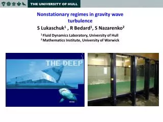
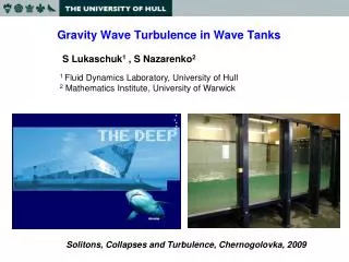
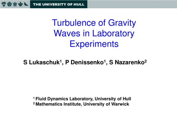
Turbulence of Gravity Waves in Laboratory Experiments. S Lukaschuk 1 , P Denissenko 1 , S Nazarenko 2. 1 Fluid Dynamics Laboratory, University of Hull 2 Mathematics Institute, University of Warwick. Plan. Introduction Experimental set-up and methods

E N D
Turbulence of Gravity Waves in Laboratory Experiments S Lukaschuk1, P Denissenko1, S Nazarenko2 1Fluid Dynamics Laboratory, University of Hull 2 Mathematics Institute, University of Warwick
Plan • Introduction • Experimental set-up and methods • Measurements of the frequency spectra and PDF for wave elevation • Comparison with numerical results and discussion • Further experiments
Theoretical prediction forsurface gravity wave Kolmogorov spectra • Kinetic equation approach for WT in an ensemble of weakly interacted low amplitude waves (Theory and numerical experiment - Hasselman, Zakharov, Lvov, Falkovich, Newell, Hasselman, Nazarenko … 1962 - 2006) Assumption: weak nonlinearity random phase (or short correlation length) spatial homogeneity stationary energy flow from large to small scales Kolmogorov spectra for gravity waves in infinite space
Phillips Spectrum Surface elevation -space: asymptotic of sharp wave crests or dimensional analysis. -space: either dimensional analysis or using Dissipation is determined by sharp wave crests (due to wave breaking) Strong nonlinearity
Finite size effects Most exact wave resonances are lost on discrete k-space (Kartashova’1991) “Frozen turbulence” (Pushkarev, Zakharov’2000) Recent numerics by Pokorni et al & Korotkevich et al (2005). To restore resonant interaction, their nonlinear brodening δmust be greater than the -grid spacing 2/L Which in our case means • >1/(kL)1/4 (Nazarenko, 2005), In numerics, this means 10000x10000 resolution for Intensity ~0.1.
Discrete scenario (Nazarenko’2005) • Ineficient cascade at small amplitudes • Accumulation of spectrum at the forcing scale until δk reaches to the k-grid spacing 2/L • Excess of energy is released via an avalanche • Mean spectrum settles at a critical slope determined by δk ~2/L, i.e. E ~ -6.
Numerical experiments • Convincing claims of numerical confirmation of ZF: A.I. Dyachenko, A.O. Korotkevich, V.E. Zakharov, (2003,2004) M. Onorato, V Zakharov et al., (2002). N. Yokoyama, JFM 501 (2004) 169–178. Lvov, Nazarenko and Pokorni (2005) • Results are not 100% satisfying because no greater than 1 decade inertial range • Phillips spectrum could not be expected in direct numerical simulations because: 1) nonlinearity truncation at cubic terms 2) artificial numerical dissipation at high k to prevent numerical blowups.
N. Yokayama (JFM, 2004) direct numerical simulationsWave action spectra
Y. Lvov, Nazarenko, Pokorni:numerical experiment: Physica D, 2006
ExperimentsAirborne Measurements of surface elevation k-spectra P.A. Hwang, D.W.Wang (2000)
Goals: Long-term: to study transport and mixing generated by wave turbulence Short-term: to characterize statistical properties of waves in a finite system Advantages of the laboratory experiment: • Wider inertial interval – two decades in k • Possibility to study both weakly and strongly nonlinear waves • No artificial dissipation – natural wavebreaking dissipation mechanism.
Total Environmental SimulatorThe Deep, Hull • 6 x 12 x 1.6 m water tank • 8 panels wave generator • 1 m3/s – flow • rain generator • PIV & LDV systems
Rain Generator 8 Panel Wave Generator Capacity Probes Laser 12 metres 90 cm 6 metres
Wave generation and measurements 2 capacitance probes at distance 40 cm\ Sampling frequency - 50-200 Hz each channel Acquisition time 2000 s
PDF of and tt PDF of is close to the Gaussian distribution around the mean value and differs at tail region, s>0, corresponds to the waves with steep tops and flat bottom. PDF of tt more sensetive to the large wavenumbers and also displays the vertical asymmetry of the wave.
N. Yokayama (JFM, 2004) direct numerical simulationsPDF of the elevation and 2
Skewness and Kurtosis for PDF of 2nd derivative of elevation
Squared amplitude of surface elevation at 6 ± 1 Hz, wire probes Probe 1 Probe 2
Conclusion Random gravity waves were generated in the laboratory flume with the inertial interval up to 1m - 1cm. The spectra slopes increase monotonically from -7 to -4 with the amplitude of forcing. At low forcing level the character of wave spectra is defined by nonlinearity and discreteness effects, at high and intermediate forcing - by wave breaking. PDFs of surface elevation and its second derivative are non-gaussian at high wave nonlinearity. PDF of the squared wave elevation filtered in a narrow frequency interval (spectral energy density) always has an intermittent tail. Questions: Which model should be used to describe our spectra?
Acknowledgement • The work is supported by Hull Environmental Research Institute