Image Processing and Sampling
Image Processing and Sampling. Aaron Bloomfield CS 445: Introduction to Graphics Fall 2006. Overview. Image representation What is an image? Halftoning and dithering Trade spatial resolution for intensity resolution Reduce visual artifacts due to quantization. What is an Image?.

Image Processing and Sampling
E N D
Presentation Transcript
Image Processing and Sampling Aaron Bloomfield CS 445: Introduction to Graphics Fall 2006
Overview • Image representation • What is an image? • Halftoning and dithering • Trade spatial resolution for intensity resolution • Reduce visual artifacts due to quantization
What is an Image? • An image is a 2D rectilinear array of pixels Continuous image Digital image
What is an Image? • An image is a 2D rectilinear array of pixels Continuous image Digital image A pixel is a sample, not a little square!
What is an Image? • An image is a 2D rectilinear array of pixels Continuous image Digital image A pixel is a sample, not a little square!
Image Acquisition • Pixels are samples from continuous function • Photoreceptors in eye • CCD cells in digital camera • Rays in virtual camera
Image Display • Re-create continuous function from samples • Example: cathode ray tube Image is reconstructed by displaying pixels with finite area (Gaussian)
Image Resolution • Intensity resolution • Each pixel has only “Depth” bits for colors/intensities • Spatial resolution • Image has only “Width” x “Height” pixels • Temporal resolution • Monitor refreshes images at only “Rate” Hz Width x Height Depth Rate NTSC 640 x 480 8 30 Workstation 1280 x 1024 24 75 Film 3000 x 2000 12 24 Laser Printer 6600 x 5100 1 - Typical Resolutions
Sources of Error • Intensity quantization • Not enough intensity resolution • Spatial aliasing • Not enough spatial resolution • Temporal aliasing • Not enough temporal resolution
Overview • Image representation • What is an image? • Halftoning and dithering • Reduce visual artifacts due to quantization
Quantization • Artifacts due to limited intensity resolution • Frame buffers have limited number of bits per pixel • Physical devices have limited dynamic range
P(x,y) I(x,y) Uniform Quantization P(x, y) = trunc(I(x, y) + 0.5) I(x,y) P(x,y) (2 bits per pixel)
Uniform Quantization • Images with decreasing bits per pixel: 256 bpp 32 bpp 8 bpp 2 bpp 8 bits 4 bits 2 bits 1 bit
Reducing Effects of Quantization • Halftoning • Classical halftoning • Dithering • Error diffusion dither • Random dither • Ordered dither
Classical Halftoning • Use dots of varying size to represent intensities • Area of dots proportional to intensity in image P(x,y) I(x,y)
Classical Halftoning Newspaper image from North American Bridge Championships Bulletin, Summer 2003
Halftone patterns • Use cluster of pixels to represent intensity • Trade spatial resolution for intensity resolution Figure 14.37 from H&B
Dithering • Distribute errors among pixels • Exploit spatial integration in our eye • Display greater range of perceptible intensities • Uniform quantization discards all errors • i.e. all “rounding” errors • Dithering is also used in audio, by the way
Floyd-Steinberg dithering • Any “rounding” errors are distributed to other pixels • Specifically to the pixels below and to the right • 7/16 of the error to the pixel to the right • 3/16 of the error to the pixel to the lower left • 5/16 of the error to the pixel below • 1/16 of the error to the pixel to the lower right • Assume the 1 in the middle gets “rounded” to 0
Error Diffusion Dither • Spread quantization error over neighbor pixels • Error dispersed to pixels right and below + + + = 1.0 Figure 14.42 from H&B
Floyd-Steinberg dithering • Floyd-Steinberg dithering is a specific error dithering algorithm Uniform Quantization (1 bit) Floyd-Steinberg Dither (1 bit) Floyd-Steinberg Dither (1 bit) (pure B&W) Original (8 bits)
P(x,y) P(x,y) I(x,y) I(x,y) Random Dither • Randomize quantization errors • Errors appear as noise P(x, y) = trunc(I(x, y) + noise(x,y) + 0.5)
Random Dither Original (8 bits) Uniform Quantization (1 bit) Random Dither (1 bit)
Ordered Dither • Pseudo-random quantization errors • Matrix stores pattern of thresholds i = x mod n j = y mod n e = I(x,y) - trunc(I(x,y)) if (e > D(i,j)) P(x,y) = ceil(I(x, y)) else P(x,y) = floor(I(x,y))
Ordered Dither • Bayer’s ordered dither matrices • Reflections and rotations of these are used as well
Ordered Dither Original (8 bits) Uniform Quantization (1 bit) 4x4 Ordered Dither (1 bit)
Dither Comparison Original (8 bits) Random Dither (1 bit) Ordered Dither (1 bit) Floyd-Steinberg Dither (1 bit)
Color dithering comparison Original image Web-safe palette, no dithering Web-safe palette, FS dithering Optimized 256 color palette Optimized 16 color palette Optimized 16 color palette FS dithering No dithering FS dithering
Summary • Image representation • A pixel is a sample, not a little square • Images have limited resolution • Halftoning and dithering • Reduce visual artifacts due to quantization • Distribute errors among pixels • Exploit spatial integration in our eye • Sampling and reconstruction • Reduce visual artifacts due to aliasing • Filter to avoid undersampling • Blurring is better than aliasing