Support Vector Machine and String Kernels for Protein Classification

Christina Leslie Support Vector Machine and String Kernels for Protein Classification Department of Computer Science Columbia University

Learning Sequence-based Protein Classification • Problem: classification of protein sequence data into families and superfamilies • Motivation: Many proteins have been sequenced, but often structure/function remains unknown • Motivation: infer structure/function from sequence-based classification

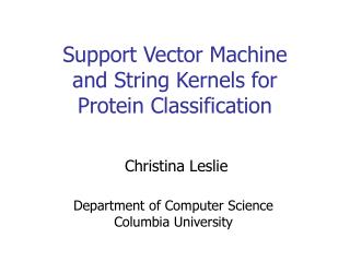
Sequence Data versus Structure and Function Sequences for four chains of human hemoglobin Tertiary Structure >1A3N:A HEMOGLOBIN VLSPADKTNVKAAWGKVGAHAGEYGAEALERMFLSFPTTKTYFPHFDLSHGSAQVKGHGK KVADALTNAVAHVDDMPNALSALSDLHAHKLRVDPVNFKLLSHCLLVTLAAHLPAEFTPA VHASLDKFLASVSTVLTSKYR >1A3N:B HEMOGLOBIN VHLTPEEKSAVTALWGKVNVDEVGGEALGRLLVVYPWTQRFFESFGDLSTPDAVMGNPKV KAHGKKVLGAFSDGLAHLDNLKGTFATLSELHCDKLHVDPENFRLLGNVLVCVLAHHFGK EFTPPVQAAYQKVVAGVANALAHKYH >1A3N:C HEMOGLOBIN VLSPADKTNVKAAWGKVGAHAGEYGAEALERMFLSFPTTKTYFPHFDLSHGSAQVKGHGK KVADALTNAVAHVDDMPNALSALSDLHAHKLRVDPVNFKLLSHCLLVTLAAHLPAEFTPA VHASLDKFLASVSTVLTSKYR >1A3N:D HEMOGLOBIN VHLTPEEKSAVTALWGKVNVDEVGGEALGRLLVVYPWTQRFFESFGDLSTPDAVMGNPKV KAHGKKVLGAFSDGLAHLDNLKGTFATLSELHCDKLHVDPENFRLLGNVLVCVLAHHFGK EFTPPVQAAYQKVVAGVANALAHKYH Function: oxygen transport

Structural Hierarchy • SCOP: Structural Classification of Proteins • Interested in superfamily-level homology – remote evolutionary relationship

Learning Problem • Reduce to binary classification problem: positive (+) if example belongs to a family (e.g. G proteins) or superfamily (e.g. nucleoside triphosphate hydrolases), negative (-) otherwise • Focus on remote homology detection • Use supervised learning approach to train a classifier Labeled Training Sequences Classification Rule Learning Algorithm

Two supervised learning approaches to classification • Generative model approach • Build a generativemodel for a single protein family; classify each candidate sequence based on itsfitto the model • Only uses positive training sequences • Discriminative approach • Learning algorithm tries to learn decision boundary between positive and negative examples • Uses both positive and negative training sequences

Hidden Markov Models for Protein Families • Standard generative model: profile HMM • Training data: multiple alignment of examples from family • Columns of alignment determine model topology 7LES_DROMELKLLRFLGSGAFGEVYEGQLKTE....DSEEPQRVAIKSLRK....... ABL1_CAEELIIMHNKLGGGQYGDVYEGYWK........RHDCTIAVKALK........ BFR2_HUMANLTLGKPLGEGCFGQVVMAEAVGIDK.DKPKEAVTVAVKMLKDD.....A TRKA_HUMAN IVLKWELGEGAFGKVFLAECHNLL...PEQDKMLVAVKALK........  

Profile HMMs for Protein Families • Match, insert and delete states • Observed variables: symbol sequence, x1 .. xL • Hidden variables: state sequence, 1 .. L • Parameters: transition and emission probabilities • Joint probability: P(x,  | )

Ladies and gentlemen, boys and girls: HMMs: Pros and Cons Let us leave something for next week …

Discriminative Learning Discriminative approach Train on both positive and negative examples to learn classifier Modern computational learning theory • Goal: learn a classifier that generalizes well to new examples • Do not use training data to estimate parameters of probability distribution – “curse of dimensionality”

Learning Theoretic Formalism for Classification Problem • Training and test data drawn i.i.d. from fixed but unknown probability distribution D on X {-1,1} • Labeled training set S = {(x1, y1), … , (xm, ym)}

Support Vector Machines (SVMs) + + • We use SVM as discriminative learning algorithm + + + • Training examples mapped to (usually high-dimensional) feature space by a feature mapF(x) = (F1(x), … , Fd(x)) _ _ + + • Learn linear decision boundary: • Trade-off between maximizing • geometric margin of the training • data and minimizing margin violations _ _ _ _

SVM Classifiers + + • Linear classifier defined in feature space by f(x) = <w,x> + b • SVM solution gives w =  ixi as a linear combination of support vectors, a subset of the training vectors + + + w _ _ b + + _ _ _ _

Advantages of SVMs • Large margin classifier: leads to good generalization (performance on test sets) • Sparse classifier: depends only on support vectors, leads to fast classification, good generalization • Kernel method: as we’ll see, we can introduce sequence-based kernel functions for use with SVMs

Hard Margin SVM + + + • Assume training data linearly separable in feature space • Space of linear classifiers fw,b(x) = w, x + b giving decision rule hw,b(x) = sign(fw,b(x)) • If |w| = 1, geometric margin of training data for hw,b S = MinSyi (w, xi + b) + + w + _ b _ _ _ _ _

Hard Margin Optimization + + + • Hard margin SVM optimization: given training data S, find linear classifier hw,b with maximal geometric marginS • Convex quadratic dual optimization problem • Sparse classifier in term of support vectors + + + + _ _ _ _ _ _

Hard Margin Generalization Error Bounds • Theorem [Cristianini, Shawe-Taylor]: Fix a real value M > 0. For any probability distribution D on X {-1,1} with support in a ball of radius R around the origin, with probability 1- over m random samples S, any linear hypothesis h with geometric margin S  M on S has error no more than ErrD(h)  (m, , M, R) provided that m is big enough

SVMs for Protein Classification • Want to define feature map from space of protein sequences to vector space • Goals: • Computational efficiency • Competitive performance with known methods • No reliance on generative model – general method for sequence-based classification problems

Spectrum Feature Map for SVM Protein Classification Newfeature map based on spectrum of a sequence • C. Leslie, E. Eskin, and W. Noble, The Spectrum Kernel: A String Kernel for SVM Protein Classification. Pacific Symposium on Biocomputing, 2002. • C. Leslie, E. Eskin, J. Weston and W. Noble, Mismatch String Kernels for SVM Protein Classification. NIPS 2002.

The k-Spectrum of a Sequence AKQDYYYYEI • Feature map for SVM based on spectrumof a sequence • The k-spectrum of a sequence is the set of all k-length contiguous subsequences that it contains • Feature map is indexed by all possible k-length subsequences (“k-mers”) from the alphabet of amino acids • Dimension of feature space = 20k • Generalizes to any sequence data AKQ KQD QDY DYY YYY YYY YYE YEI

k-Spectrum Feature Map • Feature map for k-spectrum with no mismatches: • For sequence x, F(k)(x) = (Ft (x)){k-mers t}, where Ft(x) = #occurrences of t in x AKQDYYYYEI ( 0 , 0 , … , 1 , … , 1 , … , 2 ) AAA AAC … AKQ … DYY … YYY

(k,m)-Mismatch Feature Map • Feature map for k-spectrum, allowing m mismatches: • if s is a k-mer, F(k,m)(s) = (Ft(s)){k-mers t}, where Ft(s) = 1 if s is within m mismatches from t, 0 otherwise • extend additively to longer sequences x by summing over all k-mers s in x AKQ … DKQ AKY … EKQ AAQ

The Kernel Trick • To train an SVM, can use kernelrather than explicit feature map • For sequences x, y, feature map F, kernel value is inner product in feature space: K(x, y) =  F(x), F(y)  • Gives sequence similarity score • Example of a string kernel • Can be efficiently computed via traversal of trie data structure

Computing the (k,m)-Spectrum Kernel • Use trie (retrieval tree) to organize lexical traversal of all instances of k-length patterns (with mismatches) in the training data • Each path down to a leaf in the trie corresponds to a coordinate in feature map • Kernel values for all training sequences updated at each leaf node • If m=0, traversal time for trie is linear in size of training data • Traversal time grows exponentially with m, but usually small values of m are useful • Depth-first traversal makes efficient use of memory

Example: Traversing the Mismatch Tree • Traversal for input sequence: AVLALKAVLL, k=8, m=1

Example: Computing the Kernel for Pair of Sequences • Traversal of trie for k=3 (m=0) A S1: EADLALGKAVF S2: ADLALGADQVFNG

Example: Computing the Kernel for Pair of Sequences • Traversal of trie for k=3 (m=0) A S1: EADLALGKAVF D S2: ADLALGADQVFNG

Example: Computing the Kernel for Pair of Sequences • Traversal of trie for k=3 (m=0) A EADLALGKAVF s1: D s2: ADLALGADQVFNG L Update kernel value for K(s1,s2) by adding contribution for feature ADL

Fast prediction • SVM training: determines subset of training sequences corresponding to support vectors and their weights: (xi, i), i = 1 .. r • Prediction with no mismatches: • Represent SVM classifier by hash table mapping support k-mers to weights • Test sequences can be classified in linear time via look-up of k-mers • Prediction with mismatches: • Represent classifier as sparse trie; traverse k-mer paths occurring with mismatches in test sequence

Experimental Design • Tested with set of experiments on SCOP dataset • Experiments designed to ask: Could the method discover a new family of a known superfamily? Diagram from Jaakkola et al.

Experiments • 160 experiments for 33 target families from 16 superfamilies • Compared results against • SVM-Fisher • SAM-T98 (HMM-based method) • PSI-BLAST (heuristic alignment-based method)

Conclusions for SCOP Experiments • Spectrum Kernel with SVM performs as well as the best-known method for remote homology detection problem • Efficient computation of string kernel • Fast prediction • Can precompute per k-mer scores and represent classifier as a lookup table • Gives linear time prdiction for both spectrum kernel, (unnormalized) mismatch kernel • General approach to classification problems for sequence data

Feature Selection Strategies • Explicit feature filtering • Compute score for each k-mer, based on training data statistics, during trie traversal and filter as we compute kernel • Feature elimination as a wrapper for SVM training • Eliminate features corresponding to small components wi in vector w defining SVM classifier • Kernel principal component analysis • Project to principal components prior to training

Ongoing and Future Work • New families of string kernels, mismatching schemes • Applications to other sequence-based classification problems, e.g. splice site prediction • Feature selection • Explicit and implicit dimension reduction • Other machine learning approaches to using sparse string-based models for classification • Boosting with string-based classifiers

Support Vector Machine and String Kernels for Protein Classification